Orbit simulations with Maxima software

Simulações de órbitas com o software Maxima

Abstract

The computational algebra system Maxima is used together with the fourth order Runge-Kutta method to generate simulations of orbits caused by the newtonian gravitational interaction. Such dynamical illustrations in animated GIF format, which show the trajectory of objects orbiting a much more massive attractor, are very useful to demonstrate intuitively the implications of Kepler laws. The animations are obtained with the help of the Draw package, which can use Maxima input to synthesize very customisable graphs and GIFs. Some programming tools are also necessary to this approach, once a numeric method has to be implemented in order to evaluate the orbit radius in time domain. By applying also other elements, such as variables, functions, and lists, this analysis partially shows the power of Maxima software on solving mathematical and physical problems as well as the importance of combining knowledge of Physics and programming techniques.

Keywords:
Maxima Software; Kepler laws; numeric approach; computational physics

Resumo

O sistema computacional algébrico Maxima é usado com o método de Runge-Kutta de 4^a ordem para gerar simulações de órbitas causadas pela interação gravitacional newtoniana. Tais ilustrações dinâmicas em formato de GIF animado, as quais mostram as trajetórias de objetos orbitando um atrator muito mais massivo, são muito úteis para demonstrar intuitivamente as implicações das leis de Kepler. As animações são obtidas com ajuda do pacote Draw, o qual pode utilizar os comandos do Maxima para sintetizar gráficos e GIFs altamente personalizáveis. Alguns elementos de programação são também necessários nesta abordagem, uma vez que um método numérico tem que ser implementado para a obtenção do raio das órbitas em função do tempo. Ao aplicar outros elementos, como variáveis, funções e listas, esta análise mostra parcialmente o poder do software Maxima na solução de problemas matemáticos e físicos assim como a importância de se combinar o conhecimento sobre Física e técnicas de programação.

Palavras-chave:
Software Maxima; leis de Kepler; abordagem numérica; física computacional

1. Introduction

Animations of physical systems are a very interesting didactical resource. They can be used in classes to replace static images from textbooks and classroom boards, substitute experiments, simulate phenomena which take place in very small or very large scales, show abstract objects, as vectors for example, etc. We have been using simulations in GIF format linked in our slides for some time in our classes. This made us notice that the attention and interaction of the students increase in the moments we make use of such pedagogical resources. We also have the code pieces as well as the application necessary to modify the animations in order to present different scenarios to the students or apply situations with new parameters proposed by them. Another way of presenting simulations to the students is via computer labs. In this case, the educator can point out the parameters to be modified by the students in the code pieces used to generate the animations so that they can understand the consequences of these changes in the physical situation. The GIFs can also be included in digital forms, bringing the possibility of dynamical representation of situations presented in online tests.

One large-scale phenomenon commonly discussed in Physics classes is the motion of planets, moons, asteroids, comets, and other objects in the solar system. Although orbit simulations are widely available through the Web, their customization is not always possible, once they are not usually accompanied with their generating code pieces. This can be frustrating for teachers who wish to adapt such simulations to the level of knowledge of their students, present alternative situations, or simply insert a different set of parameters in the animation. One possible way to circumvent this issue is to produce simulations by oneself [¹]. Although this brings some advantages, as the fact it helps the teacher to revisit or even to deepen his/her knowledge about the analyzed phenomena, some problems may arise, as costs of software license, programming-language complexity, etc.

We propose a solution to these issues by developing GIFs with a free computer algebra system (CAS), namely Maxima [²]. The use of open-source software is a very interesting solution specially in developing countries [³], where teachers often work with very limited resources. Nevertheless, we choose Maxima not only because it is free, but also because it possesses a tool, the Draw package, which allows the production of GIFs directly from Maxima input, without the necessity of external applications¹.

In order to illustrate the potential of Maxima software, we develop GIFs based on Kepler laws. Since the evaluation of the orbit radius in time domain demands a numeric approach in the case of non-circular orbits, this example is not only interesting to present the power of the Draw package, but also some of the main tools present in Maxima, as the programming elements such as “while”, for instance, and list manipulation commands, among others. Our idea is not to provide GIFs for educators use, but to convince them they can program their own GIFs with a free CAS. Therefore, we let our codes available at the supplementary material described in Ref. [⁵]. We use the fourth order Runge-Kutta method [⁶] to evaluate the orbit radius in time domain.

The paper is divided as follows: in section 2 we briefly revisit Kepler laws, focusing on key points necessary to develop the animations, as well as the numeric method we use to solve the differential equation related to second Kepler law; in section 3 we highlight the main Maxima tools necessary to create GIFs from numerically generated data; section 4 brings the examples we develop codes for; our conclusions are presented in section 5. We add an appendix where we analyze the precision of our results.

2. The Theory

Here we describe Kepler laws and the main equations related to them as well as the numeric method we use to obtain the evolution of the orbits with time.

2.1. Revisiting Kepler laws

Kepler laws are described in many textbooks. In Ref. [⁷], for example, first Kepler law is described as: “All planets are moving on ellipses. The sun stands in one of their focal points.” The second law reads: “The radius vector sun-planet covers equal areas in equal times (area theorem).” The third law is expressed as: “The squares of the revolution periods of two planets are related to each other as the cubes of the large semi-axes of their trajectories.”

Kepler laws can be synthesized in some formulas which we will use to develop our simulations. The first law can be expressed by the ellipse formula, which in polar coordinates is:

(1)$$r=\frac{k}{1+\epsilon \cos \theta },$$

where ε < 1 is the eccentricity, k = a(1 − ε²), with a being the large semi-axis. Equation (1) can be directly used to illustrate the figures of ellipses. However, static representations hide the fact the speed of the orbiting object changes along the trajectory, becoming faster as closer to the central attractor the object is². Therefore, such representation may be confusing for some students.

The second Kepler law can be synthesized in the following equation:

(2)$$r^2\stackrel{.}{\theta }=h,$$

where $h=\sqrt{GMk}$, with G being the gravitational constant, and M the mass of the central attractor. A dynamical representation of orbits synthesizes both the first and the second Kepler laws, as it can describe the form of the orbit at the same time it shows intuitively the speed change of the orbiting object along its trajectory. Therefore, although equation (2) may not be presented for those students who have not been introduced to calculus, it is implicitly described by the second law, which can be better presented to the students via an animation. On the other hand, teachers who wish to create simulations based on equations (1) and (2) need not only to have a profound understanding of them as well as the knowledge to code them into the CAS in order to develop their animations.

Third Kepler law is not necessary to the development of the animations, once it tell us how to compute the period of the orbit. Nevertheless, we can create animations to illustrate this law if we compare two or more orbits. We do this in Sec. 4. Furthermore, since our animations show complete orbits, it is necessary to know the direct relation between the orbit period and its large semi-axis:

(3)$$T=2\pi \sqrt{\frac{a^3}{GM}}.$$

The equations presented above depend on three parameters: a, ε, and M. We have to fix them so that our simulations may be presented in reasonable size and time. Therefore, in our codes, we choose a = 1 and GM so that T = 1³.

2.2. The numeric method

In order to generate the GIFs, we need to evaluate equation (2) in time. For this purpose, we choose the fourth order Runge-Kutta method [⁶]. Basically, if we have an equation

(4)$$\frac{dy}{dx}=f(x,y),$$

for an increment of Δx in x, we have to compute the coefficients:

(5)$$\begin{array}{l}{k}_1=f(x,y),\\ k_2=f(x+\mathrm{\Delta }x/2,y+k_1\mathrm{\Delta }x/2),\\ k_3=f(x+\mathrm{\Delta }x/2,y+k_2\mathrm{\Delta }x/2),\\ k_4=f(x+\mathrm{\Delta }x,y+k_3\mathrm{\Delta }x).\end{array}$$

Then the evolution of y is given by:

(6)$$y(x+\mathrm{\Delta }x)\approx y(x)+\left(\frac{k_1}{6}+\frac{k_2}{3}+\frac{k_3}{3}+\frac{k_4}{6}\right)\mathrm{\Delta }x.$$

The command rk in Maxima applies the fourth order Runge-Kutta method [⁸]. However, in order to make our code pieces more didactic, we implement the method using the programming tools of Maxima. This also makes easier to obtain the points necessary to trace the trajectory as the orbiting object moves in the animation.

The error of the fourth order Runge-Kutta method is of $\mathcal{O}(△x^5)$. In the orbit problem, we can also infer the errors by using the fact the orbiting object, which starts its motion in the periastron/aphastron, describes an angular displacement of π rad for each T/2 time interval. In the appendix we present the error computed in this manner for the case in which a = 1, ε = 0.5, T = 1, and Δt = 0.01.

3. Coding

In order to create graphs and GIFs from numerically generated data in Maxima it is crucial to know how to manipulate lists and to work with the Draw package. Of course one needs also to understand the basic concepts of Maxima, but we let their description to Maxima’s users manual [⁸]. Here we show some commands and options needed to manipulate lists and to model graphs and GIFs we think are necessary to the comprehension of our example codes. These code pieces have the objective of highlighting key points of Maxima and will only yield the expected results within the complete code pieces, which are available at the supplementary material, Ref. [⁵].

3.1. Lists

The main data of our numeric results are filled in lists, which Maxima stores within square brackets. These lists are used to generate the lines and dots from the numeric data in some of the figures/animations. For instance:

U : [];

creates an empty list to be filled with ordered pairs to describe the time profile of the potential energy. Inside a “while” loop we use the command “endcons”, which adds elements to a list, to populate it recursively with values of the potential energy:

U : endcons([t,-GM*m/r(th)],U),

The values of GM and m are predefined, and r(th) returns the ellipse function in polar coordinates, equation (1), with th being a variable which represents θ.

Another way to create lists is via the command “makelist”. It creates a list from a variable changing in a determined interval. For example, in our codes we make:

E : makelist([U[i][1],U[i][2]+K[i][2]], i,1,n)$

This stores elements of predefined lists of the potential and kinetic energy into a list with values of the mechanical energy⁴.

3.2. Draw package

Our main tool inside Maxima is the Draw package, which can synthesize GIFs from Maxima input without the necessity of manipulating the data in a different application environment. The description of Draw is well done in Maxima’s documentation [⁸].

Below we describe how to generate an ellipse in polar coordinates using the Draw package:

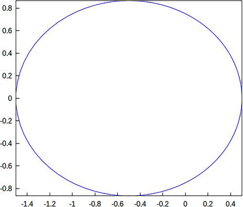
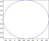
e : 0.5; /* eccentricity */ a : 1; /* major semi-axis */ k : a*(1-e^2); draw( file_name = "elipse", terminal = ’pngcairo, gr2d( nticks = 100, proportional_axes = ’xy, polar(k/(1 + e*cos(theta)), theta, 0, 2*%pi)));

Although most of the input is self-explaining, we call attention to some parts of this code piece. Here, gr2d includes the list of options to generate 2D figures. Further than “polar”, gr2d accepts other kinds of objects, as “explicit”, “points” etc. The option nticks sets the number of points used to generate the curve. Depending on the figure, we must adjust it in order to get a smoother curve. The result of the above input is shown in Figure 1.

Figure 1
The example of an ellipse generated with the Draw package. We have set a = 1 and ε = 0.5.

An example based on our codes to the orbit simulations is given below:

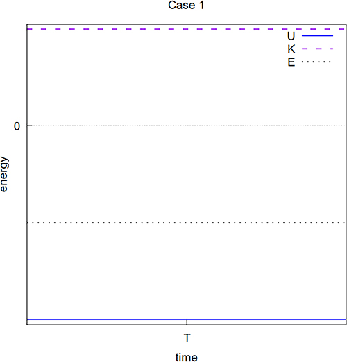
draw2d( yrange = [U[1][2]-1,K[1][2]+1], file_name = "enrg1", terminal = ’pngcairo, point_type = 0, points_joined = true, xaxis = true, xlabel = "time", xtics = {["T",1]}, ylabel = "energy", ytics = {["0",0]}, line_width = 2, title = "Case 1", key = "U", points(U), color = purple, key = "K", line_type = 2, points(K), key = "E", color = black, line_type = 3, points(E));

This is the piece of code necessary to generate the graph of the energy in the first example given in section 4. Now we use points to tell the Draw package that we want to create a curve from a list of ordered pairs of the potential, U, kinetic, K, and mechanical energy, E.

Figure 2
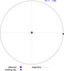
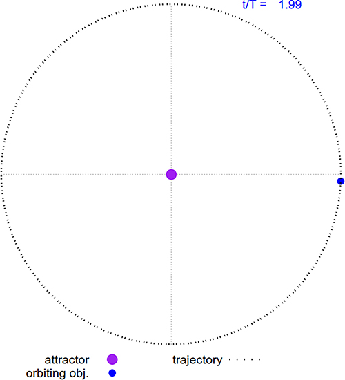
Result of the data set generated to the case of zero eccentricity. We set the time of the animation to go from t = 0 to t = 1.99T in this case. Therefore, this figure exhibits the last frame of the corresponding GIF.

Figure 3
Profile of the potential (U), kinetic (K), and mechanical (E) energy in the first case.

Let us now explain the generation of GIFs inside the Draw package. The idea is to set a list of graphs with gr2d, considering 2D animations. The draw command then synthesizes the graphs into a GIF if we specify the terminal “animated_gif”. Once again, we use the command makelist to automatize lists in which elements are logically disposed. This allows us to create smooth animations in a few lines. For example, the piece of code below creates a GIF with 100 frames of a particle describing a circular motion:

R : 1; n : 100; l : makelist(gr2d( proportional_axes = ’xy, xrange = [-R,R], yrange = [-R,R], point_type = filled_circle, points([[R*cos(t),R*sin(t)]])) ,t,0,2*%pi,2*%pi/n)$ draw( file_name = "gif_ex", terminal = ’animated_gif, l);

More complex structure can be added to the GIF, as position vector, axis projection, velocity vector, etc., as more components we add to the code. In our codes to simulate elliptical orbits, we have:

draw( file_name = "orb-ex1", terminal = ’animated_gif, makelist(gr2d( label(["t/T = ",0.5*xmax,ymax], [string(float(tm[i]/T)),0.7*xmax,ymax]), point_type = 7, point_size = 3, line_width = 2, color = purple, key = "attractor", points([[0,0]]), point_size = 2, color = blue, key = "orbiting obj.", points([pnt[i]]), color = black, points_joined = true, line_type = dots, point_type = 0, key = "trajectory", points(ipnt[i])) ,i,1,n))$

We see that most of the input serves to describe or modify parts of the graphs. The main elements here are the inputs within the brackets of points from where the points and curves corresponding to the numerically generated data are drawn. Here, pnt[i] determines the position of the orbiting object in the time t_i, which is stored in the list tm, while ipnt describes the accumulated trajectory from t = 0 to t_i.

The example presented above is used to generate one elliptical motion only. However, we can compare different motions together in the same GIF (see Sec. 4). Naturally, the code becomes more complex as more components we add to the GIF. We present the complete code pieces to generate the situations presented in Sec. 4 in the supplementary material described in Ref. [⁵].

4. Examples

Here we present some situations which we find interesting to demonstrate the power of the Draw package and Maxima in general. We consider cases which Kepler laws apply to, but with hypothetical parameters which do not represent astronomical objects from our solar system. Therefore, instead of “Sun” and “planet” used to describe Kepler laws, we use the terms “attractor” and “orbiting object” to describe our simulations. Also, we consider the case in which the attractor is much more massive than the orbiting object, so that the first can be considered at rest.

Although our main objective is to create GIFs, they cannot be disposed here. Therefore, in this paper we present only the figures relative to the considered situations while the corresponding GIFs are available at the supplementary material, Ref. [⁵].

4.1. Circular orbit

The first case is the simple case of an object in circular motion around the attractor. Although this analysis does not demand a numerical treatment, it is used as standard case to be compared with motions with considerable eccentricity. It can be also used to adjust the elements used in the graphs, such as key position, legend size, etc. Physically, it lets clear to the students that the orbiting object speed remains constant in such case. Figure 2 shows the last frame of the GIF and can be used to represent the situation statically. The corresponding GIF is available at Ref. [⁵].

The piece of code used to generate Figure 2 is presented below.

draw2d( file_name = "ex1", terminal = ’pngcairo, label(["t/T = ",0.5*xmax,ymax], [string(float(tm[n]/T)),0.7*xmax,ymax]), point_type = 7, point_size = 3, line_width = 3, color = purple, key = "attractor", points([[0,0]]), point_size = 2, color = blue, key = "orbiting obj.", points([pnt[n]]), color = black, points_joined = true, line_type = dots, point_type = 0, key = "trajectory", points(ipnt[n]));

The fact we use points indicates some of the curves/dots are plotted from numeric data. Again, most of the entries modify the format of the graph. We call the attention to the fact that the Draw package allows to set a general format to the graphs in a code. This is done by the command set_draw_defaults which we use to unify some parameters of the GIFs and figures presented here. Note that the piece of code above only generates the corresponding figure in the context of the complete code, where the necessary variables and lists are predefined.

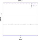
As a starting point, we also generate the graphs of the energy in this case in Figure 3. As expected, mechanical and potential energy have negative values. All kinds of energy considered hold constant as expected for circular orbits.

4.2. Elliptical orbit

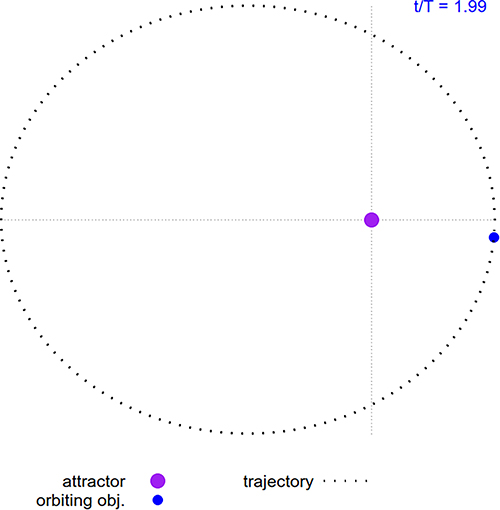
As second, we bring the case of an orbit with ε = 0.5. In this case, second Kepler law synthesizes the speed change of the orbiting object, moving faster as it approaches the periastron and slower as it approaches the apastron. The static representation of the orbit, which shows the last frame of the GIF, is shown in Figure 4.

Figure 4
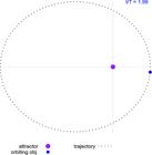
Result of the data set generated to the case of ε = 0.5. The GIF is available at the webpage described in Ref. [⁵].

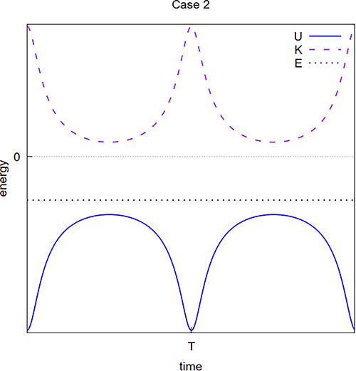
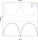
The time variation of the energy is presented in Figure 5. As expected, both E and U are negative in the entire motion. However, differently from the circular case, only E is kept constant. We can now perceive the second Kepler law via the kinetic energy once it reaches its maximum value at t = nT (n = 0, 1, 2, …) exactly in the moments the potential energy reaches its minimum value.

Figure 5
Time dependent description of the energy in case 2.

4.3. Comparison of circular orbits

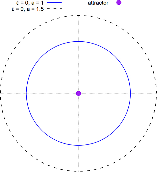
As the third case, we analyze the comparison of two circular orbits with a₂/a₁ = 1.5, where a₁ and a₂ are the large semi-axes. We neglect the interaction between the orbiting objects with each other, taking into account only their interaction with the central attractor. The idea is to make an animated example to show that planets in orbits with bigger large semi-axes take more time to complete a revolution around the attractor. At the same time, we wish to convince the reader that more orbits can be included in the simulation, generating, therefore, rich situations comparing as many orbits as the educator thinks it is necessary. The comparison of only two orbits is interesting to highlight important concepts to the students. In the present case, the key concept is the one implicit in the third Kepler law. The Maxima input also brings explicitly the ratio between the periods of both orbits, which is T₂/T₁ = 1.837.

The static scheme of the orbits comparison is shown in Figure 6. This representation is generated differently from the figures of the previous cases, as we use the orbit function in polar coordinates. The piece of code related to it is:

Figure 6
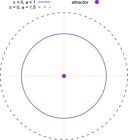
Static representation of the two-orbit simulation. This representation is generated in the same code of the simulation, so that it changes accordingly with the GIF if the initial parameters are modified.

draw2d( file_name = "ex3", terminal = ’pngcairo, key = "{/Symbol e} = 0, a = 1", polar(r(k1,e1,theta),theta,0,2*%pi), color = black, key = "{/Symbol e} = 0, a = 1.5", line_type = 2, polar(r(k2,e2,theta),theta,0,2*%pi), color = purple, key = "attractor", point_type = 7, point_size = 3, points_joined = false, points([[0,0]]));

Differently from the code presented in section 4.1, now we mix points with polar environments within draw2d. The corresponding GIF is available at the supplementary material described in Ref. [⁵].

4.4. Comparison of elliptical and circular orbits

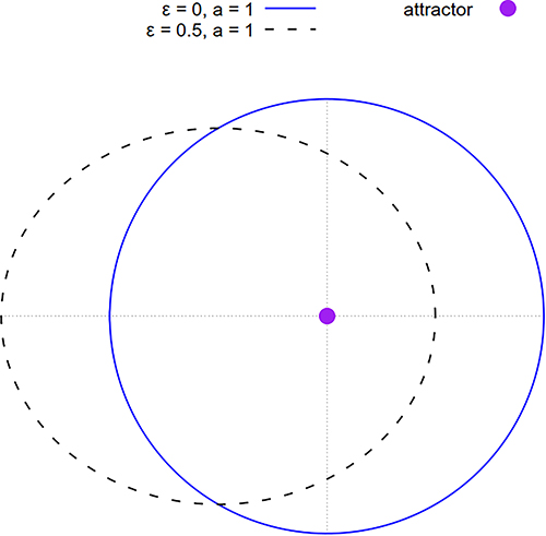
Case 4 brings the comparison of two orbits of same large semi-axis but different eccentricities, namely ε = 0,0.5. The static scheme of the comparison is presented in Figure 7. Despite their difference, the period is the same for both orbits, as expected from the third Kepler law.

Figure 7
Comparison of orbits with eccentricities ε = 0,0.5.

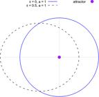
It is interesting to look at the corresponding GIF, available at Ref. [⁵], and see that the orbiting objects cross the horizontal axis at the same time although they travel in different orbits. The object in the circular orbit seems “to pass” the other object in the apastron, while the first seems to be passed by the second in the periastron. This comparison is very interesting to show the fact that the orbit period depends on the large semi-axis but not on the eccentricity.

5. Conclusions

We have carried out an analysis of Kepler laws numerically using the fourth order Runge-Kutta method. This allowed us to generate simulations of classical planetary orbits, as well as a time-domain study of the energy. Such approaches are usually not considered in basic textbooks, partially because of their limitation due to staticity, and partially because they are commonly restricted to analytical approaches.

Computers are a natural evolution in education fields, as they break the staticity of textbooks at the same time they are equipped with software which allows us to write algorithms to dynamically simulate various physical systems. Although such technological approach may possess its own limitations, such as the cost of most famous applications, we circumvent this issue by adopting Maxima, which is free software, to develop our simulations. We then remark the importance of the package Draw inside the CAS, which allows us to use Maxima input to generate GIFs without the need to export figures to another application. Such an approach may be specially interesting for educators of developing countries which have limited resources and cannot afford licenses of proprietary software.

The fact that a numerical approach is necessary to generate a time evolution of Kepler laws evidences the importance of subjects based on computational physics on teachers formation.

Once more, we call attention to the fact that our objective is not to provide GIFs of orbits, once plenty of them can be found over the Web. Since the GIFs generally available online cannot be modified, our main objective is to point out a free tool to the educators who wish to program their own animations. This may allow the teachers to highlight elements and concepts they wish to discuss with their students. Furthermore, as a CAS, Maxima may provide an initial step for those who wish to have a first contact with programming-language tools, as it possesses elements as “for”,“if”, “while”, among others, some of them included in the example codes we let available at Ref. [⁵].

Acknowledgments

This study was financed in part by the Coordenação de Aperfeiçoamento de Pessoal de Nível Superior – Brasil (CAPES) – Finance Code 001. I would like to thank L. F. S. da Silva and J. M. M. G. Holanda for useful discussions.

Supplementary Material

The following online material is available for this article:

Appendix A

Precision analysis.

Data Availability

This is a theoretical study; the generated data is not applicable for sharing.

References

• ^[1] F.J. de Almeida, Educação e informática: os computadores na escola (Cortez, São Paulo, 2012), 5 ed.
• ^[2] MAXIMA, Maxima, a Computer Algebra System, available in: https://maxima.sourceforge.io/, accessed in: 07/10/2022.
  » https://maxima.sourceforge.io/
• ^[3] N. Karjanto and H.S. Husain, Mathematics 9, 1317 (2021).
• ^[4] GNUPLOT, Gnuplot homepage, available in: http://www.gnuplot.info/, accessed in: 05/11/2022.
  » http://www.gnuplot.info/
• ^[5] E.S. de Oliveira, Orbit simulations with wxMaxima, available in: https://www.ednilton.ufpa.br/index.php/simulacoes/26-class-orbs, accessed in: 17/01/2025.
  » https://www.ednilton.ufpa.br/index.php/simulacoes/26-class-orbs
• ^[6] A. Klein and A. Godunov, Introductory Computational Physics (Cambridge University Press, New York, 2006).
• ^[7] W. Greiner, Classical mechanics: point particles and relativity (Springer-Verlag, New York, 1935).
• ^[8] MAXIMA, Maxima 5.47.0 Manual, available in: https://maxima.sourceforge.io/docs/manual/index.html, accessed in: 20/06/2025.
  » https://maxima.sourceforge.io/docs/manual/index.html
• ^[9] ejbarth, A package of maxima utilities for my ordinary differential equations course: Math280.mac, available in: https://themaximalist.org/2017/03/27/a-package-of-maxima-utilities-for-my-ordinary-differential-equations-course-math280-mac/, accessed in: 07/02/2023.
  » https://themaximalist.org/2017/03/27/a-package-of-maxima-utilities-for-my-ordinary-differential-equations-course-math280-mac/

¹

Draw itself uses Gnuplot [⁴] for default to generate graphs.

²

We consider the orbiting object with a mass much smaller than the central attractor, which can be considered at rest. We also avoid terms as “planet” and “sun” since our simulations do not have the same parameters as that of planetary motions.

³

We let the units to the reader criteria, since there are varied system scales. The period in equation (3) could represent the Moon’s orbit period, or 1 yr, but the GIF will usually have a period of seconds.

⁴

Although the mechanical energy is conserved, such definition helps to verify if the formulas have been correctly introduced into the code. We can also use these lists to help the students to visualize how the different kinds of energy change with time around the orbit.

*Correspondence email address:

[e-mail]

Editor-in-Chief:

Marcello Ferreira https://orcid.org/0000-0003-4945-3169

Publication Dates

• Publication in this collection
  29 Aug 2025
• Date of issue
  2025

History

• Received
  30 Jan 2025
• Reviewed
  26 June 2025
• Accepted
  29 June 2025