
 Multi-year capital requirements in life insurance: A stochastic mortality-based evaluation
ABSTRACT
This research aims to assess solvency capital for life insurance companies beyond the 1-year horizon, with a focus on the Brazilian Capital Framework (BCF) and Solvency II (SII), through a stochastic model using Monte Carlo simulations. Most capital frameworks apply 1-year horizons, disregarding future capital needs arising from the evolution of longevity and mortality risk, particularly under different interest rate regimes. This study incorporates a stochastic multi-year approach to bridge this oversight. By addressing long-term solvency and exploiting stochastic mortality models, this study enhances the understanding of future capital requirements and the importance of robust long-term risk management in life insurance. The findings contribute to advancing regulatory frameworks and improving the financial sustainability of the life insurance sector, particularly in preparing for extreme scenarios such as pandemics or longevity improvements. The study employs deterministic and stochastic mortality models, utilizing Monte Carlo simulations to evaluate the requirements of capital need in a multi-year horizon. It calculates capital requirements for traditional life insurance products under various scenarios, offering a comparative analysis. This study reveals that current regulatory frameworks, such as SII and the BCF, should consider extending their 1-year horizon to incorporate future capital needs not fully captured by short-term perspectives. It evaluates the capital requirement under SII and BCF using a hypothetical portfolio of 10,000 male participants for traditional life insurance products (term-life, endowment, and whole-life). Findings indicate that while it is broadly understood that lower interest rates tend to increase capital requirements, our results provide a quantitative assessment of this effect under the BCF and SII. By applying multi-year stochastic simulations, we demonstrate how changes in the interest rate environment can shift the timing and magnitude of required capital, underscoring the relevance of long-term solvency projections in regulatory analysis.
Keywords:
life insurance; Brazilian Capital Framework; Solvency II; Monte Carlo; stochastic mortality models
RESUMO
Esta pesquisa visa avaliar o capital de solvência para companhias de seguro de vida além do horizonte de 1 ano, com foco no Brazilian Capital Framework (BCF) e Solvency II (SII), por meio de um modelo estocástico utilizando simulações de Monte Carlo. A maioria das estruturas de capital aplica horizontes de 1 ano, desconsiderando necessidades futuras de capital decorrentes da evolução do risco de longevidade e mortalidade, particularmente sob diferentes regimes de taxas de juros. Este estudo incorpora uma abordagem estocástica plurianual para suprir essa omissão. Ao abordar a solvência de longo prazo e explorar modelos de mortalidade estocásticos, este estudo amplia a compreensão dos requisitos futuros de capital e a importância de uma gestão de riscos de longo prazo robusta no seguro de vida. Os achados contribuem para o avanço das estruturas regulatórias e para a melhoria da sustentabilidade financeira do setor de seguros de vida, particularmente na preparação para cenários extremos, como pandemias ou melhorias na longevidade. O estudo emprega modelos de mortalidade determinísticos e estocásticos, utilizando simulações de Monte Carlo para avaliar os requisitos de necessidade de capital em um horizonte plurianual. Ele calcula os requisitos de capital para produtos tradicionais de seguro de vida sob vários cenários, oferecendo uma análise comparativa. Este estudo revela que as estruturas regulatórias atuais, como a SII e o BCF, deveriam considerar a extensão de seu horizonte de 1 ano para incorporar necessidades futuras de capital não totalmente capturadas por perspectivas de curto prazo. Avalia o requisito de capital sob a SII e o BCF utilizando uma carteira hipotética de 10.000 participantes do sexo masculino para produtos tradicionais de seguro de vida (vida temporário, dotal e vida inteira). Os achados indicam que, embora seja amplamente compreendido que taxas de juros mais baixas tendem a aumentar os requisitos de capital, nossos resultados fornecem uma avaliação quantitativa desse efeito sob o BCF e a SII. Ao aplicar simulações estocásticas plurianuais, demonstramos como mudanças no ambiente de taxas de juros podem deslocar o momento e a magnitude do capital exigido, ressaltando a relevância das projeções de solvência de longo prazo na análise regulatória.
Palavras-chave:
seguro de vida; Brazilian Capital Framework; Solvency II; Monte Carlo; modelos estocásticos de mortalidade
1. INTRODUCTION
In actuarial science, the accurate modeling of future cash flows is indispensable for ensuring the financial sustainability of life insurance companies, pension funds, and annuity providers. These entities offer products with long-term durations, such as biometric insurance and savings-based products, which are heavily exposed to uncertainties regarding future mortality, longevity, and economic conditions. The importance of accurate modeling is recognized by both academic researchers and industry practitioners alike. Insurance companies not only rely on these models for internal purposes, such as pricing and profit testing, but also to meet stringent regulatory requirements outlined in frameworks like Solvency II (SII), the Brazilian Capital Framework (BCF), or the International Financial Reporting Standards 17 (IFRS 17). These regulations require insurers to hold sufficient capital to cover their long-term liabilities, thus protecting policyholders and maintaining market stability (Cafasso et al., 2018).
Cash-flow modeling, particularly when applied to life insurance, requires careful assumptions about future events, especially in relation to mortality rates, longevity improvements, and interest rate changes. These assumptions can be approached using two methods: deterministic and stochastic modeling. Deterministic models assume that all future events are known with certainty or are at least predictable with a high degree of confidence. In these models, all assumptions are treated as fixed inputs, leading to a single set of outcomes that reflect expected values. The key benefit of deterministic models is their simplicity; they are easy to interpret, and their results are reproducible. Each time the model is run, the same output is generated, offering a straightforward and understandable projection of future cash flows (Schmitt, 2022).
Deterministic models, while effective at capturing expected outcomes, are limited in their ability to account for variability and uncertainty, particularly in the context of long-term liabilities. They fail to adequately consider tail risks, low-probability events with high impact, such as pandemics or unexpected increases in life expectancy, which can significantly alter insurers’ liabilities. By focusing solely on average outcomes, deterministic models risk underestimating capital needs and reserve requirements, especially in extreme scenarios (Schmitt, 2022).
In contrast, stochastic models offer a more robust framework by incorporating randomness and variability into projections. These models simulate a range of potential outcomes, each with an associated probability, making them particularly suited for risks with significant uncertainty, such as mortality and longevity risk (Renshaw & Haberman, 2007). Stochastic methods, for instance, Monte Carlo simulations, generate diverse scenarios by introducing random variations in key inputs, providing a probabilistic view of future events. Widely adopted in research and practice, these models allow insurers to quantify the likelihood of different outcomes and assess tail risks that deterministic approaches overlook. For example, stochastic models can generate simulated distributions of future outcomes, enabling insurers to evaluate the financial implications of unexpected longevity improvements (Gamerman & Lopes, 2006).
The SII risk measure is the value-at-risk (VaR a ) methodology, where the capital requirement is designed to safeguard an insurance company’s own funds against a 1-in-200-year adverse event over a 1-year horizon. The BCF risk measure is the tail value-at-risk (TVaR a ) within the same 1-year horizon. This approach ensures that insurers maintain sufficient capital to retain a positive transfer value and, if necessary, to facilitate the transfer of their business.
One significant limitation of both frameworks lies in their reliance on a 1-year horizon, which inadequately captures risks with long-term implications. Systemic events, for example, may compromise the entire industry, leaving firms unable to transfer risks as intended. Similarly, prolonged risks, such as extended equity market downturns or longevity trend risks driven by gradual lifestyle changes, economic factors, or medical advancements, unfold over extended periods and are not effectively addressed within a 1-year construct. These limitations underscore the need for a closer investigation into the evolution of the capital required in the long term.
Despite significant advances in solvency regulation, the BCF and SII adopt a 1-year horizon for capital adequacy assessments. This perspective may underestimate future capital needs associated with long-term products, especially under mortality shocks or low-interest rate environments. While previous studies have explored short-term risk quantification and deterministic modeling approaches (Eling et al., 2008; Melo et al., 2011), there is a lack of research evaluating the multi-year evolution of capital requirements. This study addresses that gap by comparing capital dynamics under SII and BCF over extended horizons and by quantifying how interest rate variations and longevity trends influence the timing and size of required capital.
Hence, the primary objective of this study is to conduct a comprehensive evaluation of the capital requirements that extend beyond the standard 1-year horizon prescribed by SII and the BCF. The analysis seeks to identify and address potential future outflows whose present value may surpass the capital currently required under these regulatory frameworks, thereby highlighting risks that remain unaccounted for within the existing 1-year perspective. By exploring these overlooked capital needs, the paper aims to contribute to a more robust understanding of long-term solvency risks.
The structure of this paper is as follows: The next section introduces the literature review and analyzes various mortality models, focusing on their characteristics and underlying assumptions. In particular, we will compare discrete mortality tables with continuous mortality laws, exploring their respective advantages and disadvantages. Following this, we present stochastic mortality projections in two formats: (i) discrete mortality tables and (ii) continuous mortality laws. The final section discusses the broader implications of these models, with a particular focus on the regulatory frameworks of SII and the BCF. Recommendations are provided to enhance capital sustainability, emphasizing the importance of adopting stochastic models to better manage long-term risks and improve financial resilience.
2. LITERATURE REVIEW
The literature review will focus mainly on three areas: national regulations, international regulations, and mortality modeling.
2.1 Brazilian Regulation
The Brazilian solvency regime has evolved significantly over the past 3 decades, shifting from a framework based on simple solvency margins to a risk-based capital structure inspired by international developments such as SII and the Swiss Solvency Test. Until the mid-2010s, regulation followed what is commonly referred to as a “Solvency I” style approach. Under this model, capital requirements were largely determined by premiums written and claims retained, with little sensitivity to the specific risks embedded in insurers’ liabilities. The cornerstone of this system was Resolução do Conselho Nacional de Seguros Privados (CNSP) nº 8/1989, which introduced solvency margin rules, later revised by Resolução CNSP nº 55/2001. The framework was broadened by Resolução CNSP nº 73/2002, linking minimum capital to line of business and geographic scope.
In 2006, a regulatory package sought to strengthen supervisory control. Resoluções CNSP nº 155, 156, 157, and 158/2006 introduced rules on minimum capital, recovery plans, corrective measures, and additional capital for underwriting risk, complemented by Circular da Superintendência de Seguros Privados (SUSEP) nº 355/2007. These measures were consolidated in Resolução CNSP nº 227/2010, which offered greater coherence but preserved the fundamentally volume-based character of the system. Despite improvements, capital was still determined by deterministic criteria, meaning that companies offering long-term life and pension products faced requirements similar to those writing short-term non-life risks. As observed in the European context before SII, this lack of risk sensitivity created vulnerabilities and opportunities for regulatory arbitrage (Doff, 2008).
The decisive shift to a modern risk-based approach began in the mid-2010s. Resolução CNSP nº 321/2015 and Circular SUSEP nº 517/2015 introduced methodologies linking capital requirements to underwriting, market, credit, and operational risks. The process culminated with Resolução CNSP nº 432/2021 and Circular SUSEP nº 648/2021, which established the current BCF. This framework abandoned volume-based formulas in favor of a comprehensive, risk-sensitive methodology, aligning Brazil with international best practices (Cafasso et al., 2018).
The BCF also integrated locally calibrated biometric assumptions, most notably the Brazilian Experience Mortality Study mortality table, version 2021 (BR-EMSmt-V.2021) mortality tables (Oliveira et al., 2023). Based on the Heligman-Pollard (HP) law and reflecting national demographic data, these tables represent a significant advance over earlier frameworks, which risked miscalibration by relying on international tables. This adaptation was crucial given Brazil’s rapid increases in life expectancy and heterogeneity across regions (Instituto Brasileiro de Geografia e Estatística [IBGE], 2024).
Nevertheless, the BCF retains some limitations, also present in SII. Primarily among these is the reliance on a 1-year horizon for solvency assessment. While adequate for short-term products, this horizon is less appropriate for life and pension products, where deviations in mortality or longevity accumulate over decades. Empirical studies have shown that the 1-year perspective tends to underestimate capital needs in long-term liabilities (Rödel et al., 2021). Solvency II addresses this partially through the risk margin, calculated via a cost-of-capital method that extends the perspective to the lifetime of obligations (European Insurance and Occupational Pensions Authority [EIOPA], 2009). Brazil, however, has not introduced a comparable mechanism, which leaves its framework more exposed to short-termism.
Another limitation lies in the deterministic nature of prescribed mortality shocks. While easy to apply, these stresses do not capture the stochastic variability of mortality and longevity. The actuarial literature has shown that deterministic stress testing systematically underestimates risk, especially in tail events such as pandemics (Cairns et al., 2011). The COVID-19 crisis provided a clear illustration of the inadequacy of deterministic projections (Bastos et al., 2021).
The comparative perspective between Brazil and international frameworks underscores both convergence and divergence. Brazil has moved far beyond its former volume-based solvency regime and established a risk-based methodology consistent with global trends. At the same time, the absence of stochastic multi-year projections and of an explicit long-term adjustment mechanism leaves important gaps.
2.2 International Regulation
In line with international solvency frameworks such as SII, the BCF adopts risk-sensitive approaches to capital adequacy. However, while there has been considerable progress in aligning with these international standards, the BCF still heavily relies on deterministic models for the calculation of mortality risk (Cafasso et al., 2018). This reliance on deterministic models, which provide fixed projections of future mortality based on historical trends, presents several challenges in managing mortality risk and longevity risk, both of which are becoming increasingly significant as Brazil experiences demographic shifts toward an aging population (IBGE, 2024).
SII adopts a risk-based capital assessment, where the capital requirement is calculated using the financial measure VaR a with a = 99.5% confidence level in a 1-year horizon. In other words, insurers are required to hold enough capital to cover potential losses over 1 year with a 99.5% probability, meaning that they must be able to withstand all but the most extreme 1-in-200-year events (Eling et al., 2008). The VaR a is a function of two parameters: (i) n, the horizon, and (ii) a, the confidence level.
VaRa framework has been criticized for not being a coherent risk measure (Artzner et al., 1999) and for not accounting the long-term nature of the products (Doff, 2008), such as life insurance and pension products. The BCF adopts the same 1-year horizon and a risk measured proposed by Artzner et al. (1999), which is called by conditional tail expectation (CTE a ), well-known as tail-VaR (TVaR a ). The TVaR a is usually a coherent measure (Hull, 2021), hence is superior toVaR a .
SII requires a based on a 1 year ahead balance sheet and the solvency capital is applied to the assets (own funds).
where X is the assets cash-flow. In other words, if a company holds its own funds equal to VaR99.5% , then with probability 99.5% the loss of 1 year will not entirely consume the own funds. The VaRa ignores events beyond the quantile and therefore takes the point of view of the shareholders.
On the other hand, the TVaRa coincides with the expected shortfall (ESa ) for continuous random variables. The TVaRa admits a clear economic interpretation and it might be seen as conditional expectation of loss above the VaRa (Eq. 2).
where .
Whereas SII and the BCF consider risk over a 1-year horizon, the more recent framework of IFRS 17 is based on the fulfilment of cash flows over the whole duration of the underlying product, which requires careful consideration of an appropriate time horizon for risk quantification (England et al., 2019).
2.3 Mortality Modeling
This literature review also aims to explore the evolution of mortality models in actuarial science. We will examine both deterministic and stochastic models, highlighting their advantages and limitations, and will provide a comparative analysis of their implications for capital adequacy in the Brazilian context.
Mortality modeling, the foundation of both deterministic and stochastic approaches in life insurance, is essential for estimating mortality rates that support premium calculations, reserves, and capital requirements (Milevsky, 2022). These models are classified into discrete mortality tables and continuous mortality laws. Discrete mortality tables, widely used for pricing and reserving, provide age-specific mortality estimates but are limited in capturing trends in mortality improvements over time (Tabeau, 2001). In contrast, continuous mortality laws, such as the Gompertz and HP models, are parametric functions that offer greater flexibility. They can be calibrated to specific populations and effectively incorporate trends in longevity improvements, making them particularly valuable for long-term projections and assessing the impact of demographic changes on future liabilities (Renshaw & Haberman, 2007). For instance, the mortality table BR-EMSmt-V.2021 (Oliveira et al., 2023) uses the HP model.
The main criticism of deterministic models lies in their inability to capture mortality risk volatility and longevity risk (Cairns et al., 2011). The assumption of a fixed trajectory for mortality rates fails to recognize that future mortality rates are uncertain and subject to significant variation due to many factors, including medical advancements, pandemics, and social changes (Brouhns et al., 2002).
For instance, the COVID-19 pandemic highlighted the inadequacy of deterministic models, as they were unable to account for the sudden and unexpected changes in mortality rates caused by the global health crisis (Bastos et al., 2021). As Brazil’s population ages, with life expectancy continuing to rise, deterministic models may underestimate future survival rates, leading to inadequate capital provisions and increasing the likelihood of solvency issues (Cafasso et al., 2018).
Stochastic models, when implemented through Monte Carlo simulation, generate empirical distributions of future liabilities, enabling insurers and regulators to assess uncertainty and tail risk. This is particularly valuable for capital planning, as it allows the calculation of risk-based measures such as VaRa and TVaRa , which are integral to modern solvency frameworks like SII (Dowd et al., 2019).
In fact, the quantitative capital requirements outlined in the BCF and SII are inherently based on stochastic modeling principles. These frameworks apply risk measures to translate stochastic distributions into capital requirements. The parameterization of these models into a standard formula serves to promote consistency and usability across the insurance industry, since the standard formula reflects the risk profile of most insurance and reinsurance undertakings (EIOPA, 2009).
3. METHODOLOGY
3.1 Mortality Modeling
Mortality models are needed for determining the survival probability curve, Pr 𝑇 𝑥 ≥ 𝑡 , where Tx represents the remaining lifetime random variable of a person aged x. As previously said, there are two categories of mortality models: mortality tables and mortality laws. Typically, a conservative mortality table is used for pricing, while a suitable mortality table with potential improvement factors is set for the best estimate. Mortality laws use parametric functions to describe the mortality process of individuals within a population over a significant portion of their lifespans. An in-depth review of the key mortality laws can be found in Tabeau (2001). Some classical mortality laws are presented in Table 1, as they were designed to address various segments or the entirety of the populations under study (Pascariu, 2024).
The parameters of each mortality law are subject to constraints that ensure the biological interpretability and mathematical validity of the model. For the Gompertz law, b > 0 guarantees a well-defined exponential increase in mortality, while 𝑚∈ℝ is unrestricted. The Oppermann model requires A,C > 0 to ensure positive contributions from the infant and senescent mortality components respectively, 𝐵∈ℝ, and x > 0 to avoid the singularity at birth. For the Beard model, A,B > 0retain their Gompertz interpretation, and 𝐾≥0, where K > 0 recovers the standard Gompertz law and K > 0 implies that the force of mortality converges to the finite limit 1/𝐾 as age increases. The HP model imposes the richest set of constraints: 0 < A < 1, B, C, D, E, F, G, K > 0 and H > 1, the latter ensuring that the senescent component is strictly increasing with age. Additionally, since qx is a one-year death probability, the domain space is implicitly constrained by 0 < qx < 1 for all ages under consideration.
While deterministic mortality models rely on fixed assumptions and produce single-point forecasts, stochastic models incorporate randomness in mortality rates, enabling the generation of probability distributions for future outcomes. This added variability is essential for capturing tail risks in long-term liabilities. In this study, we adopt stochastic modeling to reflect the inherent uncertainty in mortality projections, building on the deterministic baseline typically used in regulatory capital calculations.
The mortality laws in Table 1 demonstrate direct applicability, as they were specifically designed to address distinct segments of the population. For instance, the works of Gompertz (1825) and Beard (1971) focused on modeling adult mortality, while Oppermann (1987) concentrated on infant mortality. In contrast, the mortality law proposed by Heligman and Pollard (1980) is notable for its ability to model mortality across the full age range, encompassing all stages of life.
Mortality laws offer valuable benefits by providing interpretable parameters linked to life expectancy and enabling the calculation of statistical measures such as expected value and standard deviation. For example, in the Gompertz mortality law, the parameter 𝑚 represents the modal value of the distribution in years, while b serves as a dispersion coefficient. Researchers have identified significant similarities among continuous mortality models. Hunt and Blake (2015) described an age-period-cohort (APC) model structure that encompasses most stochastic mortality models, while Currie and Schwandt (2016) demonstrate that many mortality models can be expressed using the standard framework of generalized linear or non-linear models. Building on these foundations, this section introduces the generalized APC (GAPC) family of stochastic mortality models, providing a unified approach to mortality modeling.
Let the random variable dx,cy denote the number of deaths in a population at age x last birthday during calendar year cy. Also let 𝐸 𝑥,𝑐𝑦 𝑐 denote the central exposed to risk at age 𝑥 during calendar year cy, and 𝐸 𝑥,𝑐𝑦 0 the corresponding initial exposed to risk. The force of mortality and central death rates are denoted by ux,cy and mx,cy , respectively, with the empirical estimate of the latter being
Assuming the force of mortality is constant over each year of age and calendar year, i.e., from age x to age x + 1 and year cy to cy + 1, then the force of mortality ux,cy and the death rate mx,cy coincide. This assumption is maintained throughout the analysis.
The main characteristics of the GAPC models (Hunt & Blake, 2015) are the random element and the systematic element.
The random element assumes that the number of deaths dx,cy follows a Poisson or a binomial distribution as described below:
where
These two choices for the response variable reflect the two models for the random number of deaths, dx,cy , widely used in demography and actuarial science. Under the binomial assumption, the expected number of deaths is given by .
The probability of death can therefore be estimated as the observed number of deaths divided by the initial exposure to risk, as below.
where dx,cy is the observation of the random death count.
Under the Poisson assumption, the expected number of deaths is given by , i.e., the central exposure to risk (the average number of people alive, which is used as a proxy for the total number of person-years lived) multiplied by the central mortality rate, as shown in Eq. (7).
Regarding the systematic element, this is associated with the link function nx,cy to transform the response variable (which will be some measure of mortality rates) at age x and for year cy into a form suitable for modelling and link it to the proposed predictor structure.
APC models, therefore, are the general class of generalized non-linear models, with a structure that can be written as follows:
where the first term ax is a static age function, the second term is the contribution to the mortality trend throughout the age-period terms, and the last term accounts for the cohort effect.
The link function nx,cy provides the connection between the observed data and the assumed predictor structure. In the generalized linear model framework, there are several requirements for selecting an appropriate link function. One critical requirement is that the data should be transformed to achieve an approximately linear predictor structure, rather than, for example, a multiplicative structure.
Early static and dynamic mortality models used this linearity condition as the sole criterion for choosing nx , leading to a variety of formulations, including a simplified version as proposed in Heligman and Pollard (1980)
With respect to the application of the theory to the Brazilian population, the Brazilian practice relies on periodically updated official tables. In this spirit, and following Oliveira et al. (2023), the BR-EMSmt-V.2021 mortality table was constructed by fitting the nine-parameter HP law (Heligman & Pollard, 1980). Remark that the international literature often utilizes age-period-cohort specifications to model temporal dynamics in mortality (Actuarieel Genootschap, 2024).
Let 𝜃=(𝐴,𝐵,𝐶,𝐷,𝐸,𝐹,𝐺,𝐻,𝐾) denote the HP parameters. As an illustrative exercise, we assessed whether the HP model can accurately recover meaningful parameter estimates when fitted directly to the observed mortality table, allowing for a comparison with the estimates reported by Oliveira et al. To this end, we estimate θ via nonlinear least squares using the Levenberg-Marquardt algorithm and the simplified link nx = qx , minimizing the sum of squared relative errors between the observed 1-year death probabilities from the male mortality table and the corresponding HP-implied values. The resulting fit is excellent, yielding a residual standard error of 0.0106127 on 109 degrees of freedom, which corroborates the adequacy of the HP model for representing the underlying mortality pattern. The estimated parameters, together with their standard errors, t-statistics, and associated p-values, are presented in Table 2.
In the remainder of the paper, we use the published 1-year death probabilities for males as the mortality input, rather than re-parametrizing the portfolio directly by the HP law. This choice ensures regulatory alignment and copes with extreme ages because the table represents the graduation and smoothing decisions specific to the Brazilian experience. This is in line with Brazilian supervision and practice, which conduct continuous mortality studies and publish updated official life tables. The stochastic element is implemented at the portfolio level via binomial sampling conditional on qx .
3.2 Capital Requirement Estimation
Following the previous overview of the mortality methodology, a formalization of the main concepts along with their methodology will also be presented for the capital requirements. To begin with, the expected claims and the expected statutory liabilities (reserves) t Vx are as Eq. (10) and Eq. (11-13) (see Dickson et al. [2019] for details about the definitions and standard actuarial functions and notation).
where EPV is the expected present value, t is the time in the projection horizon, SI is the sum insured, and lx is the expected population at time t.
Assuming that expenses are null and that SI = 1, for the sake of simplicity, then:
For the term-life product, the expected reserve is
where n is the term of the contract and k denotes the projection step;
For the endowment product, the expected reserve is
Finally, for the whole life product, the expected reserve is
In Eqs. 11-13, 𝑃 represents the level premium for the underlying product (term-life, endowment or whole life), represents EPV of death benefits within the remaining term, , is the EPV of the survival benefit at maturity, Ax+t is the EPV of the whole life death benefit, where EPV of future premiums and PProd represents the premium of the term-life, endowment or whole life product.
To stochastically calculate the expected claims and the expected reserve, the previous equations will be reused but considering that the number of deaths (dx ) will be binomially distributed (see Eq. 4). For each iteration (i = 1,2,... 1000), the expected number of deaths will be computed until the limiting age (𝜔=117) and then the new 𝑞 𝑥 𝑖 will be computed for that specific iteration. Table 3 summarizes the stochastic dynamics created for the 1000 iterations.
As previously mentioned, the VaR99.5% is the risk measure used in SII and the TVaR99.5% is the risk measure used in the BCF (Melo et al., 2011). In the SII context, the VaR99.5% can be translated into a 1-in-200-year (e.g., pandemic event) event that may occur, and the insurer should have enough capital to cover this event. In practice, this is the exact purpose that the capital requirement (SII or BCF) stands for and the reason why insurers need to set apart additional capital.
The Solvency Capital Requirement (SCR) and the Brazilian Capital Requirement (BCR) represent the capital that the insurance companies must set apart to comply with the SII and the BCF, respectively. Hence, the next step is to formalize those important measures that will be used in the next chapter. The BCR will be computed following the methodology in Melo et al. (2011) and described in Eq. (14):
where Prov is the expected reserve calculated using the best estimate assumptions; and the SCR was calculated by following the previous rationale and outlined in Eq. (15):
4. RESULTS
Consider a life insurance portfolio comprising n = 10,000 homogeneous male participants, all aged x = 55 at inception. The portfolio offers three distinct insurance products with a maximum premium payment period of 25 years, where premium payments cease upon death if it occurs earlier: (i) term-life insurance for 25 years, (ii) endowment insurance for 25 years, and (iii) whole-life insurance.
The sum insured for all options is S1 = 100,000. Additionally, the probability of dying in 1 year is given by qx and it is sourced from the mortality table BR-EMSmt-V.2021 male (Oliveira et al., 2023), as recommended by the regulator in Brazil. Table 4 summarizes the inputs.
The assumptions used in this study aim to balance actuarial relevance with practical feasibility. We selected age 55 as the entry age to represent a higher-risk group where the mortality rate qx is more sensitive and meaningful for capital projections. Using a much younger cohort would reduce the impact of mortality variability, while very high issue ages are uncommon in practice due to underwriting restrictions. The mortality table is the most recent standard mortality table approved by the Brazilian regulator (SUSEP), and the study was limited to male lives to simplify the interpretation.
Results will be presented for both the discrete and the continuous approaches. The stochastic mortality projections will be binomially distributed with parameters equal to the number of participants and the probability to die in 1 year (qx ) following Milevsky and Salisbury (2015).
Two ways to model the death probability (qx ) will be presented: (i) the discrete mortality table and (ii) the continuous mortality law. The last one (ii) exhibits more flexibility due to the ability to control and interpret different parameters in the model.
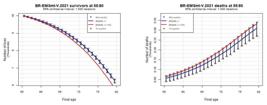
Figure 1 displays the binomial simulation of the deaths and survivors for the participants using 1,000 iterations. The quantiles 95% and 1% will be presented for each year of projection, as there will be 1,000 possible results per year. The discrete results (single result per year) using only the mortality table will be presented in the blue line to compare with the stochastic simulation. A shock in the mortality was run with an increase of 15% in the mortality, following the SII guidelines, and it is represented by the red line.
Brazilian Experience Mortality Study mortality table, version 2021 (BR-EMSmt-V.2021, ages 55-80)
From the plots on the right, it is possible to visualize the magnitude of the quantification of the mortality risk, the mortality shock, and the benefits of using stochastic analysis in comparison with the discrete approach. In the 10th year (age 65), the number of deaths could go from 79 to 150. The mean in this specific cohort is 117.3, and the expected deaths according to the mortality table are roughly equal, 117.2.
The plot on the left displays the evolution of the survivors. As expected, the number of survivors is lower in the mortality shock. Due to the range of survivors throughout the projection years, the quantiles 95% and 1% are not easy to observe.
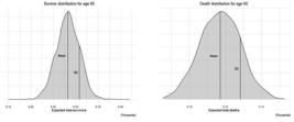
Figure 2 represents cohort 10 (or age 65) from the previous Figure 1. In other words, it shows the distribution of survivors and deaths for age 65. The shape of the plots follows a normal distribution. The mean and the first standard deviation were marked with a vertical line in the plots. Furthermore, it is possible to calculate any probabilities and empirical measures as quantiles with the distributions in Figure 2.
The plots in Figure 3 bring a quantification of some financial measures for the term-life using the given population: (i) expected claims and (ii) reserves. The left plot displays the expected total claim; the right one, the statutory liabilities (reserves). The blue line again represents expected value according to the mortality table and the red line represents the expected value according to the mortality shock in all years in the projection.
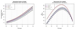
The expected claims and the statutory reserve in Figure 3 were calculated using Eq. 10. The mortality shock scenario (red line) could endanger the insurance company as it surpasses the estimated reserve. The difference could be more than 20 million in comparison with the deterministic scenario (blue line).
Figure 4 presents the loss and reserve distribution of cohort 10 (or age 65). In addition to the mean and the standard deviation, the VaR99.5% and the TVaR99.5% were pointed out with a vertical line and the area of the TVaR99.5% in green.
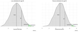
Table 5 brings important results regarding the SCR (see Eq. 15) and the BCR (see Eq. 14). The calculations only consider the life underwriting risk, as previously mentioned (see literature review). However, the required capital is more complex than this and involves different risks (e.g., market, credit, and operational) and correlations among the risks (EIOPA, 2009).
The SCR and the BCR values were calculated for the specified cohort of participants (see Table 4) over all years of the term-life insurance product, providing a vector of amounts. These values were then discounted using the risk-free interest rate term structure (estrutura a termo de taxa de juros [ETTJ]) (Associação Brasileira das Entidades dos Mercados Financeiro e de Capitais [ANBIMA], 2010). The highest discounted value within this vector, along with the corresponding time from which it was derived, is presented in Table 5 for SCR and BCR.
In addition to the ETTJ, sensitivity analyses were conducted using alternative discount rates of 0%, 1%, and 2%. The purpose of Table 5 is to compare the discounted required capital amount of each year of the entire duration at time 0 to understand when the highest amount is positioned in this vector.
Occasionally, the highest discounted value in this vector may originate from a future point in time and not from time 0. If this is the case, this observation would suggest the potential existence of a required capital need in the future that is not fully captured within the 1-year time horizon of the SII and BCF frameworks. This means that there might be a future outgo that is not being fully estimated.
The ETTJ as of November 2024 presents a time-weighted annual discount rate of approximately 6.43%. The sensitivity discount rates were intentionally set much smaller to contrast with the ETTJ and consequently produced results from different perspectives. The discount rates presented in Table 5 were sorted in increasing order.
The highest value in the discounted required capital vector at ETTJ will be 7.5 million and 8.3 million for the SCR and BCR, respectively, both values at time 0. And the highest value in the discounted required capital vector at 0% will be 9.2 million at time 18 and 10.8 million at time 15 for the SCR and BCR, respectively.
As expected, the higher the discount rate, the closer the highest value will be to time 0. Table 5 indicates that the break-even point will be higher than 2% and lower than the ETTJ (approximately 6.5%). This means that after this break-even point, the highest value will always be at time 0. The break-even point will be roughly 4.56% for the SCR and roughly 5.91% for the BCR as the vector of the BCR (TVaR99.5% ) is greater than the SCR (VaR99.5% ).
Historically, Brazil is far away from the negative or from the low-interest rate environment that the European Union was used to having, but this might be a concern in the future in Brazil. In a hypothetical scenario where the interest rate is constant and set at 0%, an insurance company would know since time 0 that it must hold 9.2 million at time 18 or 10.8 million at time 15 for the SCR and BCR respectively. However, the insurance company would only hold what is the required capital for time 0 and then top up (taking out) the incremental required capital in the subsequent years.
As the discount rate increases, the difference between the highest discounted required capital amount and the required capital at instant 0 becomes smaller until the point where the highest required capital is the one at time 0. This difference is very significant under a low-interest-rate scenario, and the 1-year horizon does not capture it, which might lead an insurance company to uncertainty.
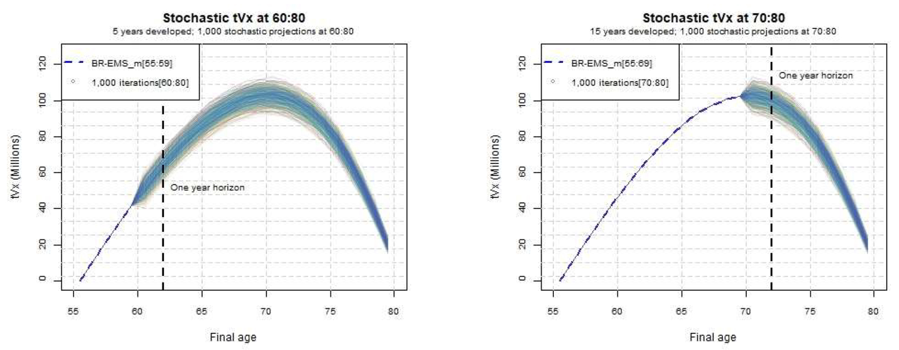
Figure 5 elaborates on this question, and it brings a picture of the 1,000 iterations in the stochastic projection at two different stages: year 5 (age 60) and year 15 (age 70) for the same term-life insurance and the referred investors. The dashed line represents the realized reserve according to the mortality table (BR-EMS_V.2021 male), and the colorful lines immediately after the dashed line represent one of the 1,000 stochastic projections until the maturity of the product. The highest uncertainty of the reserves will be observed in the years around the middle of the duration of the product in a term-life insurance.

For instance, the required capital at the end of the 5th year will be represented by the 1-year horizon (as highlighted in Figure 5) VaR99.5% of the empirical distribution of the 1,000 stochastic projections for the SCR or the TVaR99.5% of the same empirical distribution and the same 1-year horizon for the BCR.
This sheds light on the importance of properly assessing the risks that an insurance company might face using the ultimate solvency capital and sensitivity analysis scenarios. The BCF and the SII will only consider the 1-year horizon, thus ignoring the uncertainties in the future, which might be a dangerous approach.
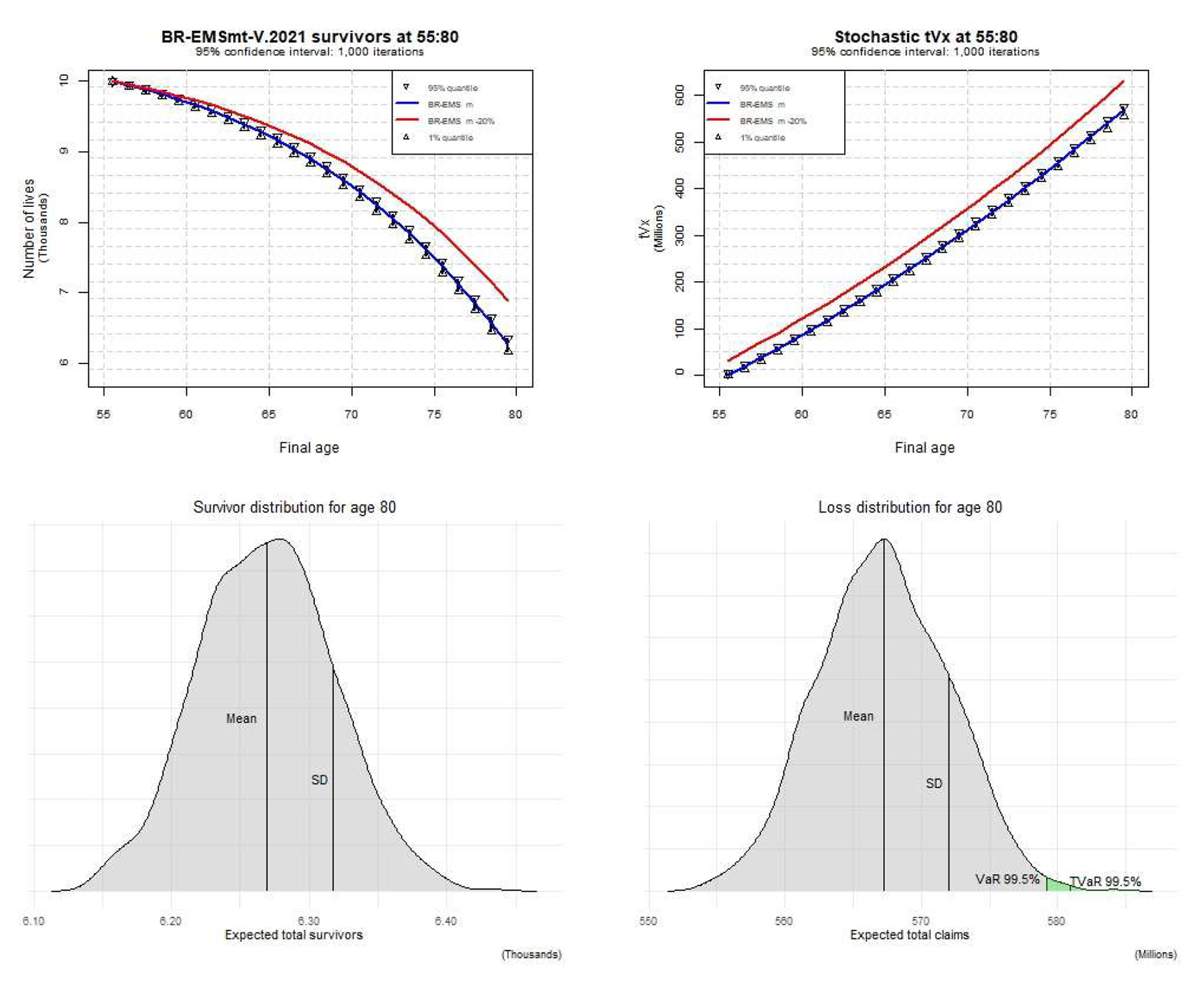
Figure 6 presents the stochastic results of the second option (endowment) and the same population. As the risk in this product is longevity (and not mortality), the stress scenario this time will be a decrease in the mortality rates by 20% according to SII.
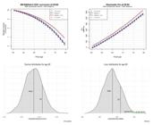
Endowment stochastics results BR-EMSmt-V.2021 = Brazilian Experience Mortality Study mortality table, version 2021.
The longevity shock can be easily observed in the survivor plot (top left). as there are more survivors expected (and fewer deaths) in the longevity shock (red line). The reserve plot displays an almost perfect linear increase that reflects the nature of this saving product, which is capital accumulation. Unlike the term-life (see Figure 3), the reserves will steadily grow until they reach the total sum insured for the expected participants alive at 80 years.
The survivor distribution at age 80 plot (bottom-left) is a snapshot at the beginning of the period, and the loss distribution for the age 80 plot (bottom-right) is a snapshot at the end of the period. Hence, the survivor distribution at age 81 plot (bottom-left) at the beginning of the period would look exactly like the loss distribution at age 80, as this is the risk inherent in this type of product. The loss distribution presents a very long tail and consequently the 𝑇 𝑉𝑎𝑅 99.5% is higher (see area highlighted in green).
Table 6 brings the results of the endowment products, and the same rationale of the elements in Table 5 was applied to this one. The highest discounted capital requirement in the vector at ETTJ (equivalent flat rate of 6.4%) will again be at time 0, and the SCR and BCR results will be, respectively, 5.9 million and 6.8 million. By decreasing the discount rate, the maximum value of the discounted cash flow will again not be at time 0 but rather at the last possible point in time.
The saving component of the endowment product drives this conclusion as the shape of the reserve is strictly increasing. The difference between the highest discounted required capital value in the vector and the required capital at instant 0 at 0% is 5.9 million (SCR) and 6.8 million (BCR). The difference at 2% decreases to 1.4 million (SCR) and 1.6 million (BCR). The gap between the highest discounted required capital in the vector and the valuation year (e.g., time 0) is too large to be completely disregarded from the methodology.
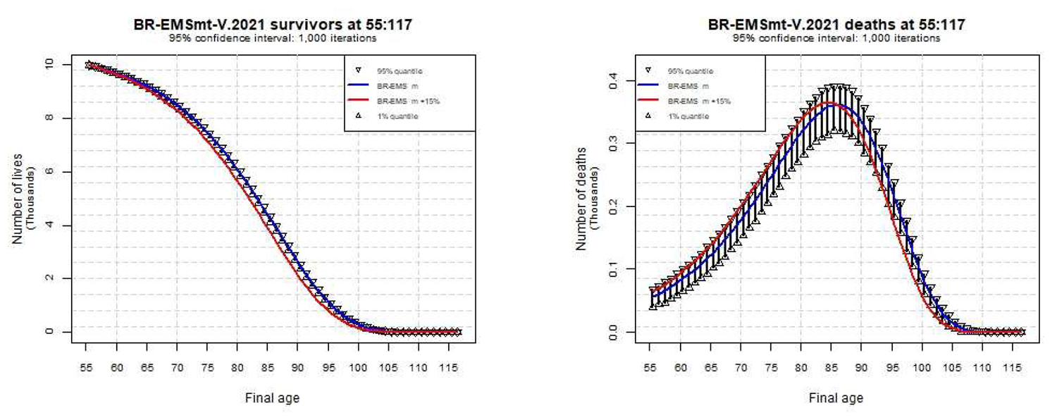
The last product is the whole life, and Figure 7 shows the evolution of the referred population of participants according to the standard and the shock scenario. The plots below are similar to Figure 1, however, with an extension until the limiting age (𝜔=117) as it is a whole-life product. The spread of the number of survivors is not easy to visualize due to the long period of projection. However, it follows the same pattern observed in the term-life product (see Figure 1).
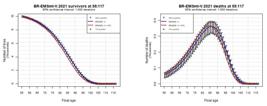
Brazilian Experience Mortality Study mortality table, version 2021, ages 55+ (BR-EMSmt-V.2021 mortality table 55+)
The evolution of the number of deaths (right plot) in the shock scenario throughout the very extensive horizon is interesting, as more deaths are expected than in the base scenario in the first half of the term, and then fewer deaths as the population is smaller (people have died before). The uncertainty after half of the term (roughly 30 years) is very large. This is reflected in the high dispersion at certain ages (80-90).
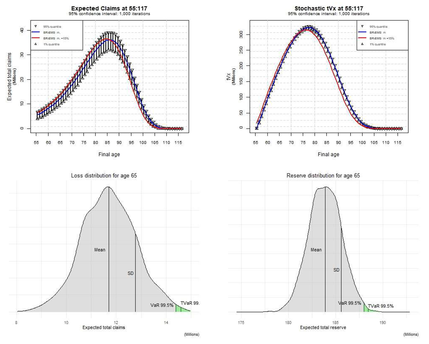
Figure 8 below displays the financial results for the whole-life product. The natural pattern of the reserve evolution in a whole-life product is a steady increase until the sum insured at the limiting age. However, the evolution of the reserves (top-right plot) is different because it is not for a single person but for the group of participants, which was initially set as 10,000. Therefore, the evolution of the reserve (right plot) will be the sum of the reserves for the expected participants alive (see Figure 7).
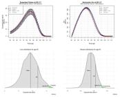
Whole-life stochastics results BR-EMS = Brazilian Experience Mortality Study; SD = standard deviation.
Loss distribution for age 65 represents the potential losses that the insurance company could have after 10 years of development of this portfolio. The mean of the loss distribution in this case is 11.7 million. However, the range of losses goes from 8.2 million to 14.7 million; thus, this is the exposure that the insurance company has in this cohort.
Finally, Table 7 presents the highest discounted capital requirement within the vector, along with the corresponding time from which it was derived for the whole-life product. The highest discounted capital requirement at ETTJ will again be at time 0. However, the same findings and conclusions obtained for the term-life and endowment products are also valid for the whole life. The highest discounted capital requirement at 0%, 1%, and 2% will be time 29, which is the middle point of the duration of this coverage.
The difference between the highest discounted capital requirement in the vector and the capital requirement at time 0 will be 4.6 million and 6.2 million, respectively, for SCR and BCR. This highlights the need to consider the long-term nature of this product instead of just analyzing 1 year ahead.
5. FINAL REMARKS
This paper highlights the critical role of stochastic mortality models in actuarial science for long-term risk assessment in life insurance. Stochastic models provide a more comprehensive understanding of risk compared to deterministic approaches, particularly for tail events like pandemics or unexpected longevity improvements. Regulatory frameworks such as SII and BCF should extend their 1-year horizon to account for the present value of potential long-term liabilities. Stress testing performed in this study (see Results) demonstrates how stochastic models yield more accurate capital estimates under adverse conditions.
By simulating mortality scenarios over extended horizons, stochastic models are vital for long-term products like life insurance, where liabilities span decades. Unlike deterministic methods, they effectively incorporate extreme events, ensuring that insurers maintain adequate capital reserves. This capacity to address tail risks makes stochastic models indispensable for enhancing the robustness of regulatory frameworks and ensuring financial stability.
To enhance capital sustainability, this study provides some recommendations. First, regulatory frameworks such as SII and BCF should promote stochastic mortality models in capital adequacy assessments. Extending the 1-year horizon to a multi-year horizon would better capture long-term risks, aligning with recommendations from Rödel et al. (2021). The BCF should also adopt stochastic models tailored to Brazil’s economic conditions, where higher volatility affects interest rates and inflation.
Second, continuous calibration of mortality models is essential to reflect evolving trends. Regular updates to methodologies like BR-EMS_V.2021 ensure that improvements in mortality are accurately captured. This study abstracts from estimating mortality time trends (APC/GAPC) and instead relies on the latest official mortality table. Incorporating external factors such as climate change, pandemics, and healthcare advancements into mortality models is critical for robust capital projections. The COVID-19 pandemic highlighted the limitations of traditional models in accounting for such shocks.
Finally, stress testing and the best estimate of liabilities in mortality models should become a core risk management practice. Advanced stochastic techniques enable insurers to simulate extreme scenarios, understand tail risks, and adjust capital allocations more effectively. This approach aligns with the SII framework, where stress testing is crucial for assessing capital adequacy.
Future research should prioritize the integration of external factors, such as lapse rate developments and advancements in healthcare, into mortality projections to further refine actuarial models. As highlighted by Atance and Navarro (2024), the growing role of technology and big data presents promising opportunities for enhancing mortality projections, offering new avenues to address the complexities of life liabilities and other long-term financial commitments.
In conclusion, the integration of stochastic mortality models into actuarial practice is not only a methodological enhancement but a necessary step for ensuring the long-term sustainability of the insurance industry. As life expectancies continue to rise and economic conditions fluctuate, the ability to accurately project future liabilities and adjust capital accordingly will be vital to the success of insurance companies globally.
REFERENCES
-
Actuarieel Genootschap. (2024). Projections life table AG 2024. https://www.actuarieelgenootschap.nl/kennisbank/projections-life-table-ag2024-1
» https://www.actuarieelgenootschap.nl/kennisbank/projections-life-table-ag2024-1 -
Artzner, P., Delbaen, F., Eber, J.-M., & Heath, D. (1999). Coherent measures of risk. Mathematical Finance, 9(3),203-228. https://doi.org/10.1111/1467-9965.00068
» https://doi.org/10.1111/1467-9965.00068 -
Associação Brasileira das Entidades dos Mercados Financeiro e de Capitais. (2010). Estrutura a termo das taxas. https://www.anbima.com.br/data/files/18/42/65/50/4169E510222775E5A8A80AC2/est-termo_metodologia.pdf
» https://www.anbima.com.br/data/files/18/42/65/50/4169E510222775E5A8A80AC2/est-termo_metodologia.pdf -
Atance, D., & Navarro , E. (2024). A simplified model for measuring longevity risk for life insurance products. Financial Innovation, 10(61). https://doi.org/10.1186/s40854-023-00515-0
» https://doi.org/10.1186/s40854-023-00515-0 -
Bastos, S., Morato, M., Cajueiro, D., & Normey-Rico, J. (2021). The COVID-19 (SARS-CoV-2) uncertainty tripod in Brazil: Assessments on model-based predictions with large under-reporting. Alexandria Engineering Journal, 60(5),4363-4380. https://doi.org/10.1016/j.aej.2021.03.004
» https://doi.org/10.1016/j.aej.2021.03.004 -
Beard, R. (1971). Some aspects of theories of mortality, cause of death analysis, forecasting and stochastic processes. In W. Brass (Ed.), Biological aspects of demography (pp. 57-68). Taylor & Francis. https://longevity-science.org/Beard-1971.pdf
» https://longevity-science.org/Beard-1971.pdf -
Brouhns, N., Denuit, M., & Vermunt, J. K. (2002). A Poisson log-bilinear regression approach to the construction of projected lifetables. Insurance Mathematics & Economics, 31(3),373-393. https://doi.org/10.1016/S0167-6687(02)00185-3
» https://doi.org/10.1016/S0167-6687(02)00185-3 -
Cafasso, P., Chela, J., & Kimura, H. (2018). The evolution of solvency regulation in Brazil: Lessons from Solvency II. Future Business Journal, 4(2),206-218. https://doi.org/10.1016/j.fbj.2018.06.005
» https://doi.org/10.1016/j.fbj.2018.06.005 -
Cairns, A., Blake, D., Dowd, K., Coughlan, G. D., & Khalaf-Allah, M. (2011). Bayesian stochastic mortality modelling for two populations. ASTIN Bulletin, 41(1),29-59. https://doi.org/10.2143/AST.41.1.2084385
» https://doi.org/10.2143/AST.41.1.2084385 -
Currie, J., & Schwandt, H. (2016). Mortality inequality: The good news from a county-level approach. Journal of Economic Perspectives 30(2), 29-52. https://doi.org/10.1257/jep.30.2.29
» https://doi.org/10.1257/jep.30.2.29 -
Dickson, D. C., Hardy, M. R., & Waters, H. R. (2019). Actuarial mathematics for life contingent risks (3rd ed.). Cambridge University Press. https://doi.org/10.1017/9781108784184
» https://doi.org/10.1017/9781108784184 -
Doff, R. (2008). A critical analysis of the Solvency II proposals. Geneva Pap Risk Insur Issues Pract, 33,193-206. https://doi.org/10.1057/gpp.2008.2
» https://doi.org/10.1057/gpp.2008.2 -
Dowd, K., Cairns, A., & Blake, D. (2019). Hedging annuity risks with the age-period-cohort two-population gravity model. North American Actuarial Journal, 25(1),170-181. https://doi.org/10.1080/10920277.2019.1652102
» https://doi.org/10.1080/10920277.2019.1652102 -
Eling, M., Gatzert, N., & Schmeiser, H. (2008). The Swiss solvency test and its market implications. Geneva Pap Risk Insur Issues Pract, 33,418-439. https://doi.org/10.1057/gpp.2008.20
» https://doi.org/10.1057/gpp.2008.20 -
England, P. D., Verrall, R. J., & Wüthrich, M. V. (2019). On the lifetime and one-year views of reserve risk, with application to IFRS 17 and Solvency II risk margins. Insurance: Mathematics and Economics, 85,74-88. https://doi.org/10.1016/j.insmatheco.2018.12.002
» https://doi.org/10.1016/j.insmatheco.2018.12.002 -
European Insurance and Occupational Pensions Authority. (2009). Directive 2009/138/EC of the European Parliament and of the Council of 25 November 2009 on the taking-up and pursuit of the business of Insurance and Reinsurance (Solvency II).https://www.eiopa.europa.eu/rulebook/solvency-ii-single-rulebook/directive-1382009ec-solvency-ii-directive_en
» https://www.eiopa.europa.eu/rulebook/solvency-ii-single-rulebook/directive-1382009ec-solvency-ii-directive_en - Gamerman, D., & Lopes, H. F. (2006). Markov chain Monte Carlo: Stochastic simulation for Bayesian inference (2nd ed.). CRC Press.
-
Gompertz, B. (1825). On the nature of the function expressive of the law of human mortality, and on a new mode of determining the value of life contingencies. Philosophical Transactions of the Royal Society of London, 115,513-583.https://www.jstor.org/stable/107756
» https://www.jstor.org/stable/107756 -
Heligman, L., & Pollard, J. H. (1980). The age pattern of mortality. Journal of the Institute of Actuaries, 107(1),49-80. https://doi.org/10.1017/S0020268100040257
» https://doi.org/10.1017/S0020268100040257 - Hull, J. (2021). Options, futures, and other derivatives (11th ed.). Pearson.
-
Hunt, A., & Blake, D. (2015). A Bayesian approach to modelling and projecting cohort effects [Discussion Paper]. Social Science Research Network. https://doi.org/10.2139/ssrn.3552217
» https://doi.org/10.2139/ssrn.3552217 -
Instituto Brasileiro de Geografia e Estatística. (2024). Tábuas completas de mortalidade para o Brasil - 2023.https://biblioteca.ibge.gov.br/visualizacao/periodicos/3097/tcmb_2023.pdf
» https://biblioteca.ibge.gov.br/visualizacao/periodicos/3097/tcmb_2023.pdf -
Melo, E., Neves, C., Altieri, E., & Cardoso, P. (2011). Modelo padrão de cálculo do capital adicional baseado no risco de subscrição de seguro de vida individual e previdência. Revista Brasileira de Risco e Seguro, 7,1-38.https://www.rbrs.com.br/arquivos/rbrs_13_1.pdf
» https://www.rbrs.com.br/arquivos/rbrs_13_1.pdf -
Milevsky, M. A. (2022). How to build a modern tontine: Algorithms, scripts and tips. Springer International Publishing. https://doi.org/10.1007/978-3-031-00928-0
» https://doi.org/10.1007/978-3-031-00928-0 -
Milevsky, M. A., & Salisbury , T. S. (2015). Optimal retirement income tontines. Insurance: Mathematics and Economics , 64,91-105. https://doi.org/10.1016/j.insmatheco.2015.05.002
» https://doi.org/10.1016/j.insmatheco.2015.05.002 -
Oliveira, M. de, Bertho, A. C. S., Costa, B., Sommerlatte Silva, F., Alves, M. B., Ramos Ramirez, M., Borges, R. B. de R., Marques, R., Rosa, R. M. da S., Peregrino, R. L., Lobo, V. das G. R., & Fonseca, T. C. O. (2023). Tábuas de mortalidade BR-EMS 2021 do mercado segurador brasileiro. Revista Brasileira de Estudos de População, 40, 1-24. https://doi.org/10.20947/S0102-3098a0252
» https://doi.org/10.20947/S0102-3098a0252 - Oppermann, L. (1987). On the graduation of life tables, with special application to the rate of mortality in infancy and childhood. The Insurance Record: Minutes from a Meeting in the Institute of Actuaries, 42.
-
Pascariu, M. D. (2024). MortalityLaws: Parametric mortality models, life tables and HMD [R package]. R Project. https://cran.r-project.org/web/packages/MortalityLaws/index.html
» https://cran.r-project.org/web/packages/MortalityLaws/index.html -
Renshaw, A. E., & Haberman, S. (2007). On simulation-based approaches to risk measurement in mortality with specific reference to Poisson Lee-Carter modelling [Research Paper]. Faculty of Actuarial Science & Insurance. https://openaccess.city.ac.uk/id/eprint/2313/
» https://openaccess.city.ac.uk/id/eprint/2313/ -
Rödel, K. T., Graf, S., & Kling, A. (2021). Multi-year analysis of solvency capital in life insurance. European Actuarial Journal, 11,463-501. https://doi.org/10.1007/s13385-021-00259-0
» https://doi.org/10.1007/s13385-021-00259-0 -
Schmitt, M. (2022). Derivation of biometrically dependent cash flows. European Actuarial Journal, 12,779-812. https://doi.org/10.1007/s13385-021-00303-z
» https://doi.org/10.1007/s13385-021-00303-z -
Tabeau, E. (2001). A review of demographic forecasting models for mortality. Forecasting Mortality in Developed Countries, 9,1-32. https://doi.org/10.1007/0-306-47562-6_1
» https://doi.org/10.1007/0-306-47562-6_1
-
This is a bilingual text. This article has also been translated into Portuguese, published under the DOI https://doi.org/10.1590/1808-057x20252285.pt
-
DATA AVAILABILITY STATEMENT
Datasets related to this article will be available upon request to the corresponding author.
-
GENERATIVE AI DISCLOSURE
The authors declare that no generative artificial intelligence was used in any stage of the production of this manuscript (including research, writing, data analysis, formula generation, or the creation of graphic elements).
Datasets related to this article will be available upon request to the corresponding author.

 Source: Elaborated by the authors.
 Source: Elaborated by the authors.
 Source: Elaborated by the authors.
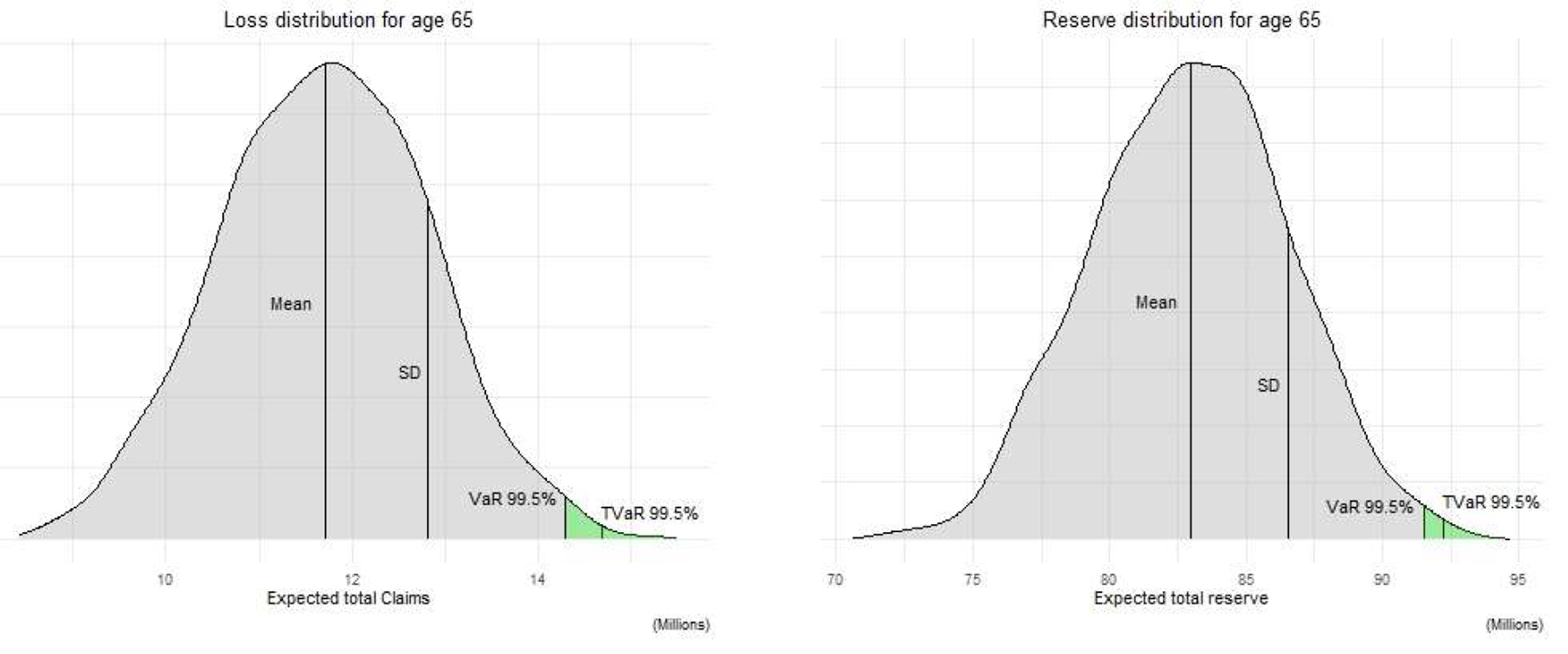 Source: Elaborated by the authors.
 Source: Elaborated by the authors.
 Source: Elaborated by the authors.
 Source: Elaborated by the authors.
 Source: Elaborated by the authors.