Spontaneous period-doubling cascade and chaos

Abstract

The simulation, in flow regime, of the chlorate-nitrous acid-iodine-iodide oscillating reaction has shown a new kind of dynamic behavior. In addition to bursts separated by increasing amplitude oscillations, at low input chlorate concentration and low flow rate a repetitive sequence of bifurcations presenting period-1 (regular oscillations), period-2 (double amplitude oscillations), period-4 (four amplitude oscillations), etc., followed by chaos, which is a period-doubling cascade, was observed. This sequence of bifurcations and chaos occurs between a cluster of bursts. However, this sequence of bifurcations, chaos and bursts occur spontaneously and keeps repeating without the change of any parameter of the system, which are the input concentrations and flow rate.

Key words
complexity; bifurcations; period-doubling; chaos; bursts; oscillating reactions

INTRODUCTION

Complexity is a science which has many facets (Goldenfeld & Kadanoff 1999). It connects with chemistry, physics, mathematics, biology, economy, climate, nervous system, fractals, epidemiology, and many other general or specific areas. In chemistry, complexity is related to clock reactions, oscillating reactions, spontaneous pattern formation (Turing structures), chemical waves, and chaos (Gray & Scott 1990, Epstein & Pojman 1998, Semenov et al. 2016, Kondepudi & Prigogine 1998, Field & Burger 1985, Vidal & Pacault 1984). In addition, oscillating reactions may present different rhythms and oscillating patterns, depending on the participation of fast and slow inhibitors (Wang et al. 2023). A recently discovered chlorate-nitrous acid-iodine-iodide oscillating reaction (Monteiro et al. 2021) has shown different burst patterns and rhythms, in flow regime, by measuring the absorbance at 460 nm. Simulation of this oscillating reaction by numerical integration has shown some of the oscillation patterns observed experimentally, most of them bursts, but also other complex burst patterns not yet observed experimentally. One of these patterns presents a repetitive bifurcation sequence formed by a period-1 (regular oscillations), period-2 (double amplitude oscillations), period-4 (four amplitude oscillations), etc., which is a period-doubling cascade, followed by chaos, and followed by a cluster of bursts. This pattern repeats over and over again, without the change of any parameter. This pattern is a very special dynamic behavior never seen before.

MATERIALS AND METHODS

Numerical integrations were performed using two different methods: a) Runge-Kutta integration method codified in Turbo Pascal; b) MATLAB ode15s numerical integration method. The Appendix presents the MATLAB scripts used in this work. Upon request, the authors can provide critical parts of the Turbo Pascal code. Chemical details of the mechanism of the chlorate-nitrous acid-iodine-iodide oscillating reaction are presented below (see Chemical Details section), including the calculation of the absorbance at 460 nm.

Runge-Kutta numerical Integration

In this case, a semi-implicit fourth order Runge-Kutta integration method was used (Kaps & Rentrop 1979), employing the constants set GRK4A (see Kaps & Rentrop 1979, Table 3.27). The use of the constants set GRK4T (see Kaps & Rentrop 1979, Table 3.28) produced similar results, but computations took a little longer. This was the numerical integration method which allowed us to discover the new dynamic behavior presented in this work. The mechanism shown in the Chemical Details section, was converted to a system of differential equations, each one corresponding to a different independent chemical species, and codified in Turbo Pascal (Gábor et al. 2015). This was the numerical integration method used to calculate the phase portrait and the cluster of four bursts presented in the Results and Discussion section. We have been using this integration method, codified in Turbo Pascal, for a long time and we used this same method recently to simulate the photochemical chlorate-iodide clock reaction (Pires & Faria 2022). Numerical extended precision of the Turbo Pascal, which uses 10 bytes, corresponding to 19 to 20 significant digits, allowing to represent real numbers in the range 3.4 × 10-4932 to 1.1 × 104932, was used for all variables. All numerical integrations were made using a tolerance equal to 1 × 10-3. The use of a small tolerance equal 1 × 10‑4 did not change the results, but it made the integration slower.

MATLAB ode15s numerical Integration

To check the results obtained by the Runge-Kutta method codified in Turbo Pascal, we used the ode15s solver for stiff differential equations, available in the MATLAB package (The Mathworks, Inc. 2022). This approach has also been used by other authors to simulate oscillating reactions (Stanisavljev et al. 2023). In this case, numerical precision is not as high as in Turbo Pascal. All variables are internally represented in double precision, which uses 8 bytes, allowing them to represent real numbers in the range 2.22 × 10-308 to 1.79 × 10308. The MATLAB ode15s solver was used with the options RelTol = 1 × 10-12, AbsTol = 1 × 10-12, NormControl = on, and InitialStep = 1 × 10-15. Reducing the option RelTol to 1 × 10-9 does not change significantly the results and the calculated patterns were the same produced by the use of semi-implicit fourth order Runge-Kutta integration method codified in Turbo Pascal. However, when using RelTol equal to 1 × 10-7 the results degrade, presenting a mix of clusters of bursts made by one, two, three, and four bursts, and also the pattern between the clusters of bursts changes to mostly chaotic. The Appendix presents the MATLAB scripts “reaction_runfile_RF3_0005.m” and “mechanism_RF3_0005.m” which can be used to reproduce the results presented in this work using MATLAB.

Calculating the phase portrait and the oscillating patterns

To build the phase portrait presented in the Results and Discussion section, no continuation method was used. All borders of this diagram were determined by a careful step by step change in the k₀ value. With respect to the oscillation patterns, the results presented in this work were obtained after a long integration time at fixed values of all input concentrations and k₀. It means and must be understood that they are not transient results. To be sure that they are not transient results we integrated using a long-time scale and the final values of all variables were used as starting values for another long-time integration session. Only after the same pattern was observed to be the same in more than two long-time sequential integrations, we considered that the pattern is stabilized, and it is reproducible. To make easy to check if a pattern is stable, the code in line 38 of the MATLAB script “reaction_runfile_RF3_0005.m” reads the final concentrations of the last integration and code in line 49 save the final concentrations after the ode15s solver has been called (see the Appendix).

It is also worth mentioning that to obtain the results shown in the Results and Discussion section, it was necessary, sometimes, to increase the k₀ value by very small amounts (in the range of 1 × 10-6 s-1 and in a few cases 1 × 10-7 s-1), step-by-step, otherwise the system jumps to a steady state or to a different behavior, as it is well known to occur with any complex system. In addition, to observe the patterns shown in the Results and Discussion section we start from a steady state using a low k₀ value, outside the oscillation region indicated in the phase portrait. Then, increasing k₀ by small amounts it is possible to observe, initially, regular oscillations. If we keep increasing k₀ the bursts start to appear. Of course, as indicated above, after one numerical integration session, the final values of all variables must be saved to be used as the starting variable values for the next numerical integration session, using the same k₀ value, to check if the behavior is not a transient one. Only after checking that the behavior is not a transient behavior the k₀ is changed to a slightly higher value.

Chemical details

Chemical details of the oscillating reaction simulated in this work, in flow conditions, are presented below. From the mathematical point of view, all chemical species are parameters and variables of the system. The chemical reactions which were translated into differential equations to be integrated by numerical methods, are presented in Table I. In this way, Table I presents the mechanism of the chlorate-nitrous acid-iodine-iodide oscillating reaction (Monteiro et al. 2021) simulated in this work. It is based on the mechanism used to simulate the photochemical chlorate-iodide clock reaction (Pires & Faria 2022), which is an expansion of the mechanism proposed by Lengyel, Li, Kustin, and Epstein to simulate the behavior of the chlorine dioxide/chlorite-iodide reaction (Lengyel et al. 1996). To the mechanism of the photochemical chlorate-iodide clock reaction we added the reactions involving nitrogen species (reactions M27-M34), and we decreased the rate constant for reaction M17. As the reactions M19 and M21 include the participation of light, and reaction M27 involves the participation of oxygen, it is a mechanism for a photochemical oscillating reaction running in flow regime (CSTR- continuously feed stirred tank reactor) in a reactor open to the atmosphere. Considering that this oscillating reaction can be followed at 460 nm, where the main absorption species are iodine (ε = 740 L mol-1 cm-1) and triiodide ion (ε = 972 L mol-1 cm-1), the calculated absorbance was computed from the calculated concentrations of these species obtained by numerical integration, multiplied by their respective molar absorptivity (Rábai & Beck 1987, Palmer & Van Eldik 1986).

Table I
Mechanism of chlorate-nitrous acid-iodine-iodide oscillating reaction

Label	Reaction	Rate law*
M1(a)	ClO2• + I- → ½ I2 + ClO2-	6×103[ClO2•][I-]
M2a(a)	I2 + H2O ⇄ HOI + I- + H+	1.98×10-3[I2]/[H+] - 3.67×109[HOI][I-]
M2b(a)	I2 + H2O ⇄ I- + H2IO+	5.52×10-2[I2] - 3.48×109[H2IO+][I-]
M3(a)	HClO2 + I- + H+ → HOI + HOCl	7.8[HClO2][I-]
M4(h)	HClO2 + H2IO+ → HIO2 + HOCl + H+	2×105[HClO2][H2IO+]
M5(a)	HClO2 + HIO2 → IO3- + HOCl + H+	1×106[HClO2][HIO2]
M6(a)	HOCl + I- → HOI + Cl-	4.3×108[HOCl][I-]
M7(a)	HOCl + HIO2 → IO3- + Cl- + 2 H+	1.5×103[HOCl][HIO2]
M8(a)	HIO2 + I- + H+ ⇄ 2 HOI	1×109[HIO2][I-][H+] - 22[HOI]2
M9(a)	2 HIO2 → IO3- + HOI + H+	25[HIO2]2
M10(a)	HIO2 + H2IO+ → IO3- + I- + 3 H+	110[HIO2][H2IO+]
M11(a)	Cl2 + H2O ⇄ HOCl + Cl- + H+	22[Cl2] - 2.2×104[HOCl][Cl-][H+]
M12(a)	Cl2 + I2 + 2 H2O → 2 HOI + 2 Cl- + 2 H+	1.5×105[Cl2][I2]
M13(a)	Cl2 + HOI + H2O → HIO2 + 2 Cl- + 2 H+	1×106[Cl2][HOI]
M14(a)	HClO2 ⇄ ClO2- + H+	2×108[HClO2] - 1×1010[ClO2-][H+]
M15(a)	H2IO+ ⇄ HOI + H+	3.4×108[H2IO+] -1×1010[HOI][H+]
M16(a)	I2 + I- ⇄ I3-	5.6×109[I2][I-] - 7.5×106[I3-]
M17(b)	ClO3- + H2IO+ → HIO2 + HClO2	6×104[ClO3-][H2IO+][H+]
M18(c)	ClO3- + Cl- + 2 H+ → ClO2• + ½ Cl2 + H2O	3.86×10-6[ClO3-][Cl-][H+]3
M19(h)	I- + H2O + hν → I• + H• + OH-	2.08×10-3[I-]
M20(d)	I• + I• → I2	8×109[I•]2
M21(h)	I2 + hν → I• + I•	1×10-3[I2]
M22(h)	H• + H• → H2	1×109[H•]2
M23(h)	H• + I• → H+ + I-	1×108[H•][I•]
M24(e)	HIO3 ⇄ H+ + IO3-	1×108[HIO3] - 3.125×108[H+][IO3-]
M25(e)	H+ + I- + HIO3 ⇄ I2O2 + H2O	1×107[H+][I-][HIO3] - 1×108[I2O2]
M26(e)	I- + H+ + I2O2 → I2 + HIO2	4.67×108[I-][I2O2] + 6.29×1010[I-][I2O2][H+]
M27(f)	2 NO• + O2 → 2 NO2•	2.1×106[NO•]2[O2]
M28(f)	NO• + NO2• ⇄ N2O3	1.1×109[NO•][NO2•] - 3.7×104[N2O3]
M29(b)	H2NO2+ ⇄ HNO2 + H+	2×106[H2NO2+] - 1×108[HNO2][H+]
M30(b)	H2NO2+ + I- ⇄ NOI + H2O	6×104[H2NO2+][I-] - 6×10-1[NOI]
M31(b)	NOI + I- → NO• + I2•-	1×106[NOI][I-]
M32(b)	I2•- + H2NO2+ → NO• + I2 + H2O	1×108[I2•-][H2NO2+]
M33(f,g)	2 HNO2 ⇄ N2O3 + H2O	1.5×10-6[HNO2]2 - 1×103[N2O3]
M34(b)	ClO3- + H2NO2+ → NO3- + HClO2 + H+	1.8×10-2[ClO3-][H2NO2+]

• *Rate parameters units are s-1, L mol-1 s-1, L2 mol-2 s-1, L3 mol-3 s-1 for first-, second-, third-, and forth-order reactions, respectively. (a) Lengyel et al. 1996; (b) This work; (c) Sant’Anna et al. 2012; (d) Kimura et al. 1991; (e) Csekö et al. 2019; (f) Lewis & Deen 1994; (g) Dózsa et al. 1976; (h) Pires & Faria 2022.

RESULTS AND DISCUSSION

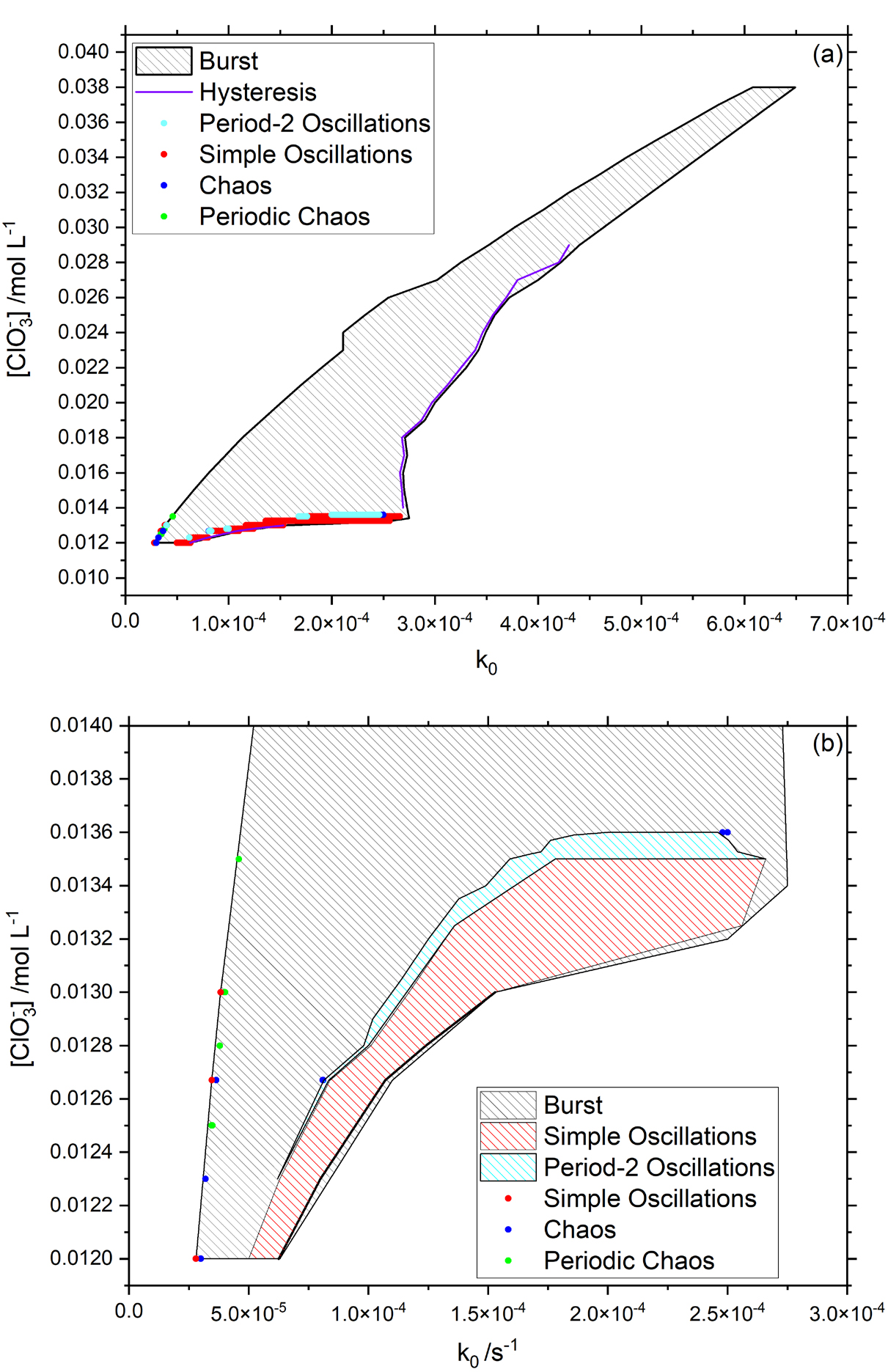
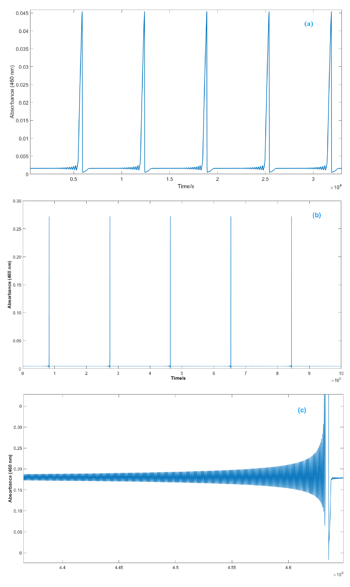
A general view of the results is shown by the phase portrait in Figure 1. As indicated in this figure, inside the closed region, bursts separated by increasing amplitude oscillations is the most common behavior. The time which separates the bursts and the number and amplitude of increasing amplitude oscillations between them, depend on the parameters values (chlorate concentration and flow rate (k₀)), as can be seen in Figure 2.

Figure 1
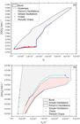
Phase portrait for the chlorate-nitrous acid-iodine-iodide oscillation reaction. [HNO₂] = 1.60 × 10-3 mol L-1, [I₂] = 2.74 × 10-4 mol L-1, [I-] = 8.40 × 10-3 mol L-1, [O₂] = 2.58 × 10-4 mol L-1, [H+] 2.0 × 10-2 mol L-1. (a) Full scale; (b) Detail at low chlorate concentration.

Figure 2
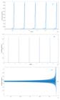
Bursts with increasing amplitude between them. [HNO₂] = 1.60 × 10-3 mol L‑1, [I₂] = 2.74 × 10-4 mol L-1, [I-] = 8.40 × 10-3 mol L-1, [O₂] = 2.58 × 10-4 mol L-1, [H+] 2.0 × 10-2 mol L‑1, (a) [ClO₃‑] = 1.25 × 10-2 mol L‑1, k₀ = 3.540 × 10-5 s-1; (b) [ClO₃-] = 3.00 × 10-2 mol L‑1, k₀ = 3.752 × 10-4 s-1; (c) detail of (b).

As shown in the lower part of the phase portrait (see the window in Figure 1b), other dynamic behaviors can be seen, depending on the parameter values (chlorate initial concentration and flow rate (k₀)): i) simple oscillations (period-1 oscillations); ii) period-2 oscillations; iii) bursts (which can appear as a single burst or a cluster of bursts containing two, three, etc. bursts; iv) a repetitive spontaneous change of behavior, without change of any parameter, presenting a period-doubling cascade (period-1, period-2, period-4, and so on) followed by chaos and a cluster of bursts, which it is indicated as Periodic Chaos, which means that the system presents a chaotic behavior which appears and disappears periodically. In other words, each green point in Figures 1a and 1b corresponds to a sequence of different behaviors that change spontaneously to the next behavior at a fixed value of chlorate initial concentration and also a fixed value of flow rate (k₀).

Different dynamic behaviors, such as regular oscillations, period-doubling cascade, chaos, and bursts, as a consequence of a parameter change, is a phenomenon well known (Epstein & Pojman 1998, Field & Burger 1985, Roux at al. 1983). However, a spontaneous change of behavior, without the change of any parameter, in the best of our knowledge, has not been reported before.

The simulation results we present in this work for the chlorate-nitrous acid-iodine-iodide oscillating reaction (Monteiro et al. 2021) consider the inflow concentrations of chlorate, nitrous acid, iodine, iodide, dissolved oxygen, H+, and the flow rate (k₀) as parameters. The calculated concentrations of all chemical species in the reaction mixture, each one as a function of time, are the responses of the system, as well the absorbance at 460 nm, which depends on the calculate concentrations of iodine and triiodide ion, as explained in the Materials and Methods section. However, it is worth mentioning that a detailed discussion of the chemistry of this system is not the intention of this article. The focus of the present work is to present a new dynamic behavior discovered by chance. The concentrations of the chemical species and k₀ are the mathematical variables and parameters of a complex system which shows, as far we know, a new dynamic behavior, we call Periodic Chaos, i.e. a chaotic behavior that happens periodically.

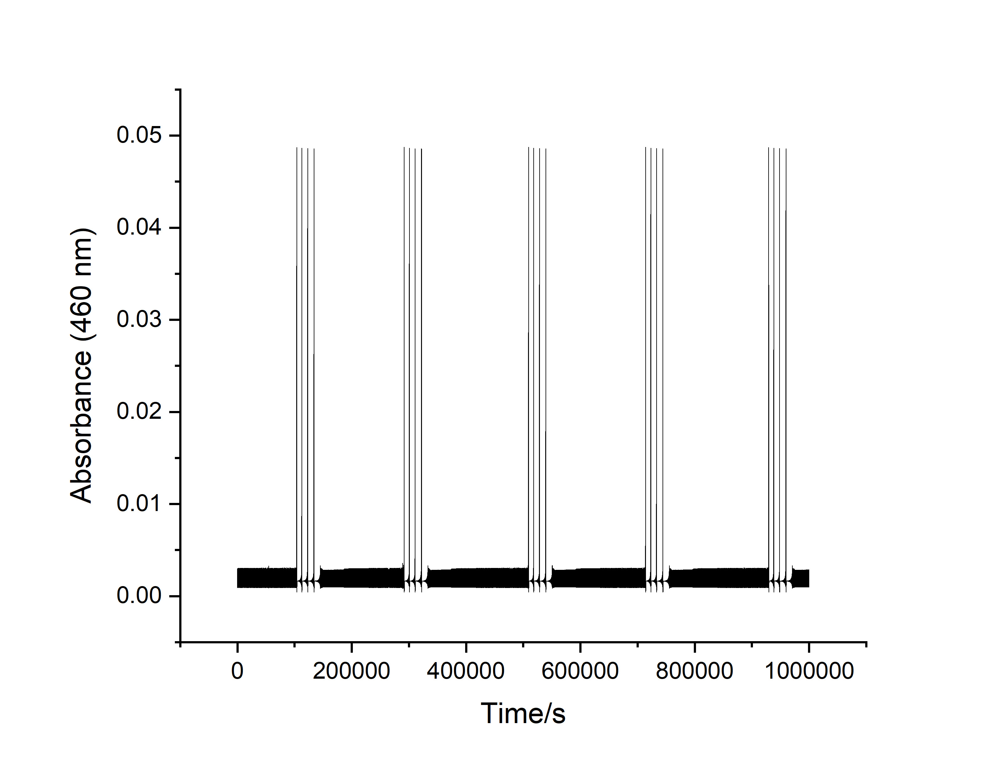
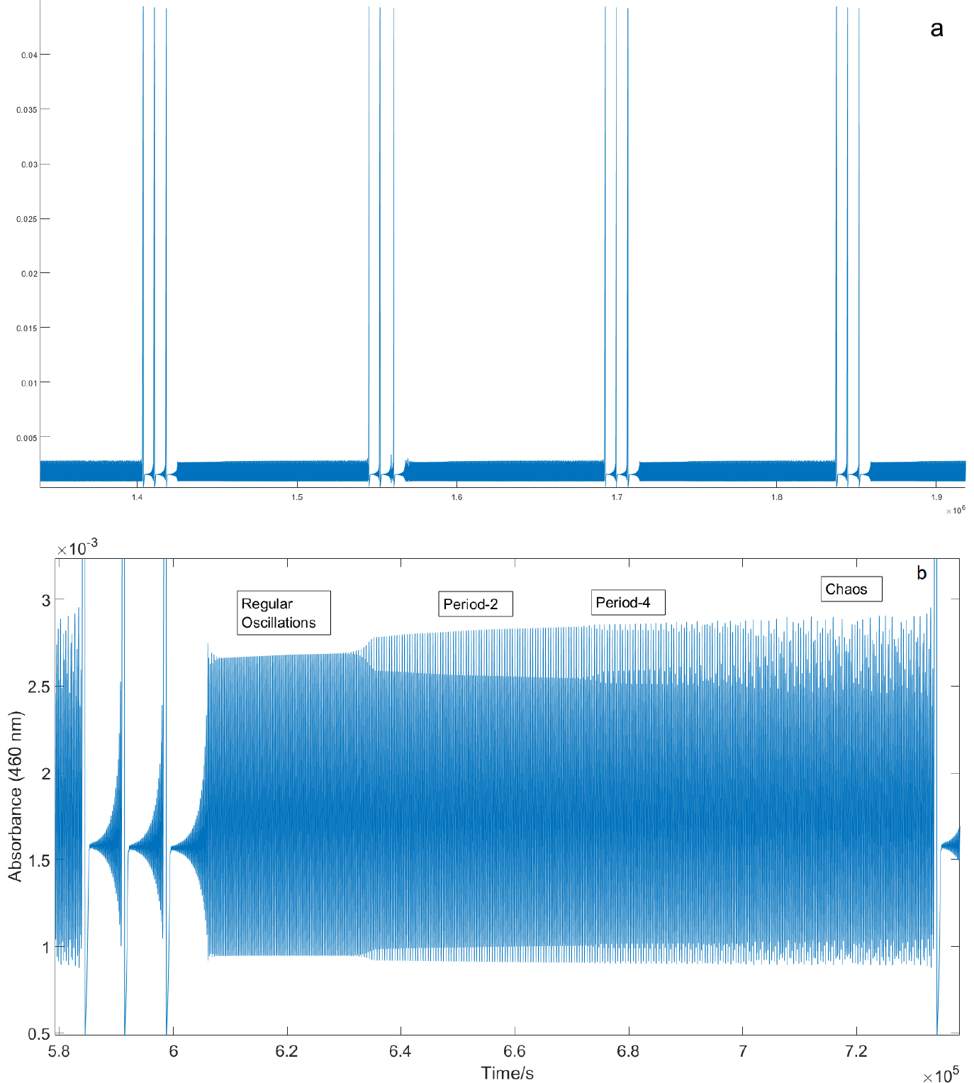
The Periodic Chaos appears between clusters of bursts in a small window of parameters: 1.25 × 10-2 mol L-1 < [chlorate] < 1.35 × 10-2 mol L-1 and 3.5 × 10-5 s-1 < k₀ < 4.6 × 10-5 s-1. At [chlorate] = 1.30 × 10-2 mol L-1 and k₀ = 3.98420 × 10-5 s-1 we observe clusters of four bursts, as can be seen in Figure 3. Clusters of three bursts can be seen at [chlorate] = 1.25 × 10-2 mol L-1 and k₀ = 3.44662 × 10-5 s-1 (Figure 4a). These clusters of bursts have some similarity with the cluster of bursts found by other authors (Sørensen 1974, Rinzel & Troy 1982, Dolnik & Epstein 1993). However, a closer look in the region between each cluster of bursts shows a new dynamic behavior. As can be seen in Figures 3 and 4a, there are a huge number of small oscillations between each cluster of bursts. As can be seen in more detail in Figure 4b, as time goes, initially, after the cluster of three bursts, the system presents regular oscillations (period-1), which, after some time, spontaneously, changes to period-2, and then to period-4, and finally to chaos, without any change in parameters. After spending some time in the chaotic regime, a cluster of three bursts starts again and all the sequence repeats forever, as the system is in a flow regime in a CSTR. The same behavior is found between the clusters of four bursts shown in Figure 3.

Figure 3
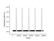
Clusters of four bursts. [ClO₃-] = 1.30 × 10-2 mol L-1, [HNO₂] = 1.60 × 10-3 mol L-1, [I₂] = 2.74 × 10-4 mol L-1, [I-] = 8.40 × 10-3 mol L-1, [O₂] = 2.58 × 10-4 mol L-1, [H+] = 2.0 × 10-2 mol L-1, k₀ = 3.98420 × 10-5 s-1.

Figure 4
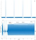
Clusters of three bursts. [ClO₃-] = 1.25 × 10-2 mol L-1, [HNO₂] = 1.60 × 10-3 mol L-1, [I₂] = 2.74 × 10-4 mol L-1, [I-] = 8.40 × 10-3 mol L-1, [O₂] = 2.58 × 10-4 mol L-1, [H+] = 2.0 × 10-2 mol L-1, k₀ = 3.44662 × 10-5 s-1. (a) full vision; (b) detail of oscillations between the clusters of bursts.

As described in the Materials and Methods section, we employed two different numerical integration methods to verify if this new behavior is not related to mathematical precision or numerical integration method. As a result, we observed the same patterns in the same range of parameters for both numerical integration methods, indicating that they are not a mathematical artifact.

Regarding to the chaotic behavior at the end of the period-doubling cascade shown in Figure 4b, several methods can be used to identify the presence of chaos, for example: a) calculating Liapunov exponents; b) drawing a two-dimensional projection of the attractor by the time delay method; c) drawing a next-amplitude map (Lorenz map); d) drawing a Poincaré section; e) drawing a next-return map from a Poincaré section; f) Fourier power spectrum analysis (Epstein & Pojman 1998, Strogatz 2015, Scott 1991).

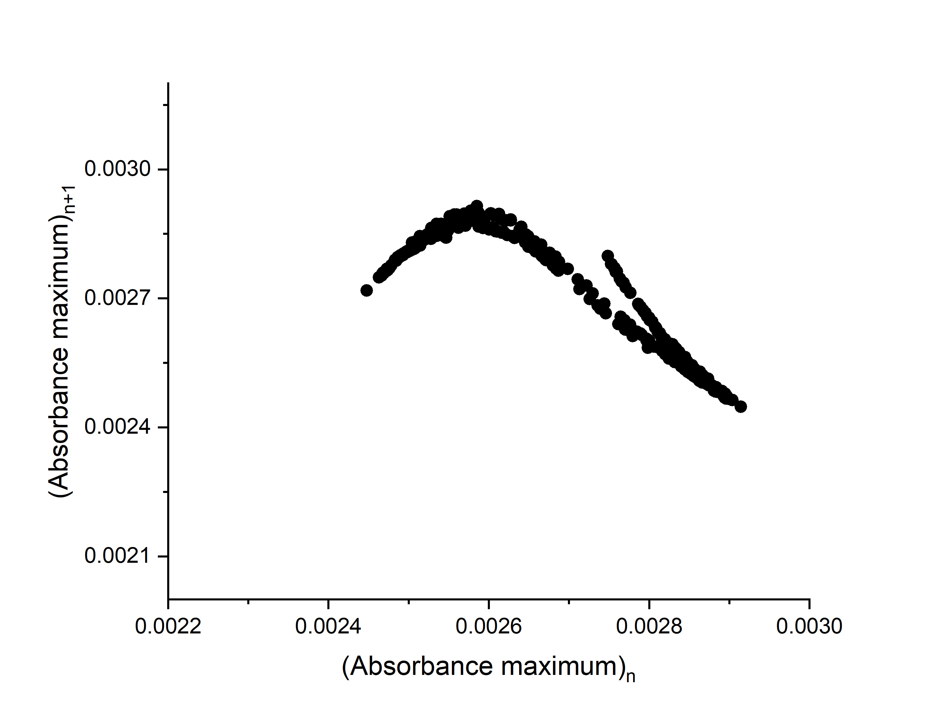
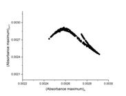
Applying the next-amplitude map (Lorenz map) to the Regular Oscillations region indicated in Figure 4b produced, as expected, a single point for the plot of the maximum absorbance versus the maximum absorbance of the next oscillation. For the Period-2 region we obtained two separated points, indicating that the system bifurcated, spontaneously, without any change of parameters, to a period-2 oscillations. As the time goes, the system bifurcates again, spontaneously, to a short-term Period-4 oscillations, indicated by a blurred four points in the next-amplitude map for this small period of time, and for the final region, labeled Chaos, before the cluster of three bursts starts again, we obtained a next-amplitude map which does not show any cluster of points, as shown in Figure 5, indicating a chaotic behavior.

Figure 5
Next-amplitude map for the chaotic region indicated in Figure 4b.

Chaotic behavior has been known since long time ago. Theoretical models like Lorenz (1963) and Rössler (1976) are iconic and have been much studied. Chemical systems which show chaotic behavior have also been known since a long time ago, being the Belousov-Zhabotinsky system one of the most studied (Roux et al. 1983, Schmitz et al. 1977), and some kinetic models for this reaction have been able to simulate the chaotic behavior observed experimentally (Györgyi et al. 1991).

Chaos and chaotic behavior have attracted much attention, and there are many books and articles on this theme. Some of these works consider chaotic behavior from the point of view of complexity (Gleick 1987, Mitchell 2009), philosophic consequences (Prigogine 1997), mathematical point of view (Strogatz 2015, Ott 1993), and connections with chemical systems (Strogatz 2015, Scott 1991, Showalter & Epstein 2015). However, in all these cases, when a system behaves in a chaotic fashion, it is chaotic all the time. For example, in the famous Lorenz model, the observed behavior depends on the values of three parameters, σ (Prandt number), r (Rayleigh number), and b (Strogatz 2015). If these parameters have values equal to 10, 28, and 8/3, respectively, this mathematical system presents a chaotic behavior. Chaotic behavior is not restricted to these exact values. For example, it occurs in the range 24.74 < r < 99.524 (Strogatz 2015). But without change of σ, r, or b, the system does not change its behavior. On the other hand, the behavior shown in Figure 4b, which presents a repetitive sequence of different behaviors, including chaos, without any change in the parameters, has not been observed before.

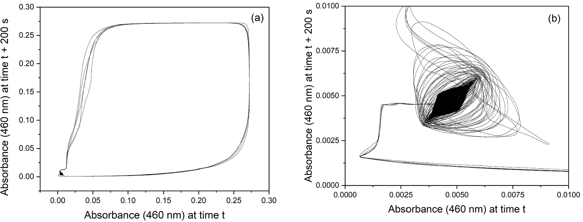
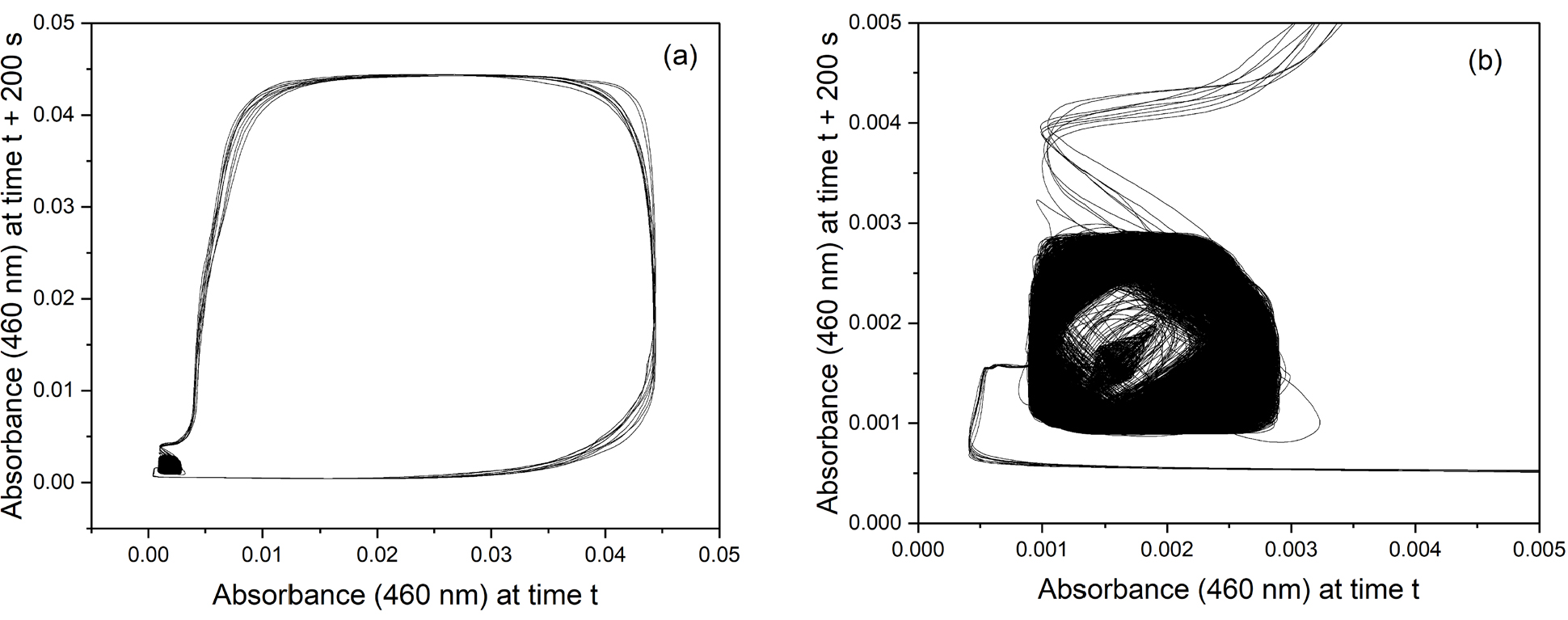
In addition to the next-amplitude map, analysis of complex behaviors can also be made by drawing a two-dimensional projection of the attractor by the time delay method, as indicated above. Figure 6 shows a projection of the attractor for the behavior shown in Figures 2b and 2c, using Δt = 200 s. The large orbits in Figure 6a correspond to each burst and the packaged orbits in Figure 6b correspond to the increasing amplitude oscillations shown in detail in Figure 2c. Similarly, Figure 7 shows the two-dimensional projection of the attractor for the behavior shown in Figure 4, using the same Δt = 200 s. Again, the large orbits in Figure 7 correspond to the bursts.

Figure 6
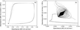
Attractor for the behavior shown in Figures 2b and 2c, using Δt = 200 s. (a) Full vision; (b) Detail corresponding the increasing oscillations before the burst. [HNO₂] = 1.60 × 10-3 mol L‑1, [I₂] = 2.74 × 10-4 mol L-1, [I-] = 8.40 × 10-3 mol L-1, [O₂] = 2.58 × 10-4 mol L-1, [H+] 2.0 × 10-2 mol L‑1, [ClO₃-] = 3.00 × 10-2 mol L‑1, k₀ = 3.752 × 10-4 s-1.

Figure 7
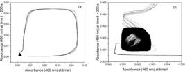
Attractor for the behavior shown in Figure 4, using Δt = 200 s. (a) Full vision; (b) Detail corresponding the period-doubling cascade followed by chaos, before the cluster of bursts. [HNO₂] = 1.60 × 10-3 mol L‑1, [I₂] = 2.74 × 10-4 mol L-1, [I-] = 8.40 × 10-3 mol L-1, [O₂] = 2.58 × 10-4 mol L-1, [H+] 2.0 × 10-2 mol L‑1, [ClO₃-] = 1.25 × 10-2 mol L‑1, k₀ = 3.44662 × 10-5 s-1.

Comparison between Figures 6b and 7b shows a significant difference. The congested orbits shown in Figure 6b correspond to the increasing amplitude oscillations that precede each burst (see Figure 2c). On the other hand, the congested region shown in Figure 7b presents a dense ring formed by many close orbits, indicating a chaotic behavior. In addition, in the center of this ring, we can see a less congested region of orbits, which looks like Figure 6b, corresponding to the period-doubling cascade which precedes the chaotic behavior.

The comparison above between Figures 6b and 7b supports that Figures 3 and 4 presents a new behavior, which is a repetitive sequence of period-doubling cascade, followed by chaos, inside a cluster of bursts, without any change of parameters.

Tracking the concentration of the chemical species (the response of the system) during different moments of the complex behavior shown in Fig. 4b, can give some inside about the processes responsible for this behavior. In doing this we observed that:

i) Cl-, IO₃-, ClO₃-, HIO₃, HNO₂, and H₂NO+ species do not change significantly their concentrations during bursts or between them.

ii) O₂ and ClO₂• increase their concentrations during the period-doubling cascade and chaotic behavior but decrease at each burst event. This suggests that these species trigger each burst when their concentrations are higher than a threshold value. When their concentrations are low, no burst occurs.

iii) Concentrations of N₂O₃ and concentrations of the radicals NO•, NO₂•, I•, and H• do not change significantly during the period-doubling cascade and chaos but change significantly in the burst events.

iv) Concentrations of I₂O₂, NOI, I₂•-, I-, and I₃- change in a low range of values, during the period-doubling cascade, chaos, and bursts (1 × 10-16 to 1 × 10-6 mol L-1).

v) Concentrations of I₂, HOCl, HIO₂, HClO₂, ClO₂-, Cl₂, HOI, and H₂IO+, also change during the period-doubling cascade, chaos, and bursts, but in a higher range of values (1 × 10-8 to 1 × 10-4 mol L-1).

As in the case of the photochemical chlorate-iodide clock reaction (Pires & Faria 2022), HOI, H₂IO+, HIO₂, and HClO₂ are the main autocatalytic species responsible for oscillations and burst. In addition to these autocatalytic species, the present system also involves very reactive free radicals, I•, H•, I₂•-, NO•, and NO₂•, which participate in reactions with very high rate-constant values. As indicated above, NO•, NO₂•, I•, and H• change significantly their concentrations in the burst’s events. This suggests that the peak of absorbance shown in the bursts is a consequence of fast reactions involving these radicals, which produce and consume iodine and triiodide ion very rapidly. In this way, we consider that the presence of these very reactive radicals is another key factor, in addition to the presence of autocatalytic species, which make the complexity of this system still higher, in such a way to produce the behavior shown in Figures 3 and 4.

CONCLUSIONS

A new dynamic behavior was observed in the simulation of an oscillating reaction, which presents a repetitive period-doubling cascade followed by chaos, inside a cluster of bursts, without any change of parameters. This new behavior (see Figures 3 and 4) occurs in a narrow range of the parameters chlorate concentration and flow rate. The time scale for the oscillations and bursts observed in this simulation is different from the time scale of oscillations and bursts observed in laboratory for this chemical system (Monteiro et al. 2021). Although the behavior shown in Figures 3 and 4 has not been observed experimentally until now, it is a new dynamic behavior which opens a window to be explored in simulations and warns experimentalists about this possibility.

The reason for the emergence of this new behavior can be speculated. It looks like there are, at least, two main processes occurring on a very different time scale. One of them is responsible for the bursts and the increasing amplitude oscillations between them. The other is responsible for producing the bifurcation sequence (a period-doubling cascade followed by chaos), which has a role like a repetitive change of a parameter’s value (for example, k₀). Both processes must be in phase to produce the behavior shown in Figures 3 and 4 and this may explain why the parameters’ range is narrow.

It is also possible that the presence of slow and fast reactions, running simultaneously and interconnected, can be a requirement to produce this new behavior. In other words, there is a possibility that this new behavior can be observed only in complex systems containing many variables and reactions (differential equations), otherwise, this would have been observed previously in smaller systems. In this way, it can be viewed as an emergent behavior, which can be observed only in systems containing a minimal number of variables and differential equations. A small version of the present system is certainly desirable. However, if it is an emergent behavior which occurs only for systems with minimal number of variables, reduction of this system to a small one may prevent observing this new behavior.

Real systems like, for example, an isolated neuron, neurons networks, the brain, the immune system, a single cell or a multicell superior being, are systems which contain a huge number of processes running in parallel and interconnected. In this way, it is not improbable that the behavior shown in Figures 3 and 4 will be observed in future in natural systems or in huge mathematical models, such as the models used to forecast weather and climate, for example.

Acknowledgements

We thank Dr. Istvan Lengyel for the use of his Turbo Pascal code to make the simulations by numerical integration. We also thank the financial support from Ministério da Ciência, Tecnologia e Inovações − MCTI and Conselho Nacional de Desenvolvimento Científico e Tecnológico − CNPq (Grant 305.737/2022-8 (RBF)). This study was financed in part by the Coordenação de Aperfeiçoamento de Pessoal de Nível Superior - Brasil (CAPES) - Finance Code 001.

• Data availability
  Data will be made available upon reasonable request.

References

• CSEKÖ G, GAO Q, XU L & HORVÁTH AK. 2019. Autocatalysis-Driven Clock Reaction III: Clarifying the Kinetics and Mechanism of the Thiourea Dioxide-Iodate Reaction in an Acidic Medium. J Phys Chem A 123: 1740-1748.
• DOLNIK M & EPSTEIN IR. 1993. A coupled chemical burster: The chlorine dioxide–iodide reaction in two flow reactors. J Chem Phys 98: 1149-1155.
• DÓZSA L, SZILASSY I & BECK M. 1976. Mechanism of the nitrite-iodide reaction. Inorg Chim Acta 17: 147-153.
• EPSTEIN IR & POJMAN JA. 1998. An Introduction to Nonlinear Chemical Dynamics: Oscillations, Waves, Pattern and Chaos. New York: Oxford University Press, 408 p.
• FIELD RJ & BURGER M. 1985. Oscillations and Traveling Waves in Chemical Systems. New York: Wiley, 682 p.
• GÁBOR B, MULLER P & VREMAN P. 2015. Free Pascal IDE, version 1.0.12.
• GLEICK J. 1987. Chaos - Making a new science. New York: Viking Press, 310 p.
• GOLDENFELD N & KADANOFF LP. 1999. Simple Lessons from Complexity. Science 284: 87-89.
• GRAY P & SCOTT SK. 1990. Chemical oscillations and instabilities: non-linear chemical kinetics. New York: Oxford University Press, 453 p.
• GYÖRGYI L, REMPE SL & FIELD RJ. 1991. A novel model for the simulation of Chaos in Low-Flow-Rate CSTR Experiment with the Belousov-Zhabotinsky Reaction: A Chemical Mechanism for Two Frequency Oscillations. J Phys Chem 95: 3159-3165.
• KAPS P & RENTROP P. 1979. Generalized Runge-Kutta methods of order four with stepsize control for stiff ordinary differential equations. Numer Math 33: 55-68.
• KIMURA M, OHOMURA A, NAKAZAWA F & TSUKAHARA K. 1991. Kinetics and Mechanisms of Photo-Induced Reduction of Iodine by Diamine-N- polycarboxylate Ions in an Aqueous Solution. Bull Chem Soc Jpn 64: 1872-1877.
• KONDEPUDI D & PRIGOGINE I. 1998. Modern Thermodynamics. From Heat Engines to Dissipative Structures. Chinchester: John Wiley & Sons, 486 p.
• LENGYEL I, LI J, KUSTIN K & EPSTEIN IR. 1996. Rate constants for reactions between iodine-and chlorine-containing species: a detailed mechanism of the chlorine dioxide/chlorite-iodide reaction. J Am Chem Soc 118: 3708-3719.
• LEWIS RS & DEEN WM. 1994. Kinetics of the reaction of nitric oxide with oxygen in aqueous solutions. Chem Res Toxicol 7: 568-574.
• LORENZ EN. 1963. Deterministic Nonperiodic Flow. J Atmos Sci 20: 130-141.
• MITCHELL M. 2009. Complexity - A guided tour. Oxford: Oxford University Press, 349 p.
• MONTEIRO EV, QUEIROZ JPR & FARIA RB. 2021. The chlorate-nitrous acid-iodine-iodide oscillating reaction. ACS Omega 6: 7959-7965.
• OTT E. 1993. Chaos in Dynamic Systems, 2nd ed., Cambridge: Cambridge University Press, 478 p.
• PALMER D & VAN ELDIK R. 1986. Spectral Characterization and Kinetics of Formation of Hypoiodous Acid in Aqueous Solution. Inorg Chem 25: 928-931.
• PIRES RO & FARIA RB. 2022. The Photochemical Chlorate-Iodide Clock Reaction. Inorg Chem 61: 1178-1187.
• PRIGOGINE I. 1997. The end of certainty. Time, chaos, and the new laws of the nature. New York: Free Press, 240 p.
• RÁBAI G & BECK MM. 1987. Kinetics and Mechanism of the Autocatalytic Reaction between Iodine and Chlorite Ion. Inorg Chem 26: 1195-1199.
• RINZEL J & TROY WC. 1982. Burstin phenomena in a simplified Oregonator flow system model. J Chem Phys 76: 1775-1789.
• RÖSSLER OE. 1976. An equation for continuous chaos. Phys Lett 57A: 397-398.
• ROUX JC, SIMOYI RH & SWINNEY HL. 1983. Observation of a strange attractor. Phys D 8: 257-266.
• SANT’ANNA RTP, SANTOS CMP, SILVA GP, FERREIRA RJR, OLIVEIRA AP, CÔRTES CES & FARIA RB. 2012. Kinetics and Mechanism of Chlorate-Chloride Reaction. J Braz Chem Soc 23: 1543-1550.
• SCHMITZ RA, GRAZIANI KR & HUDSON JL. 1977. Experimental evidence of chaotic states in the Belousov-Zhabotinskii reaction. J Chem Phys 67: 3040-3044.
• SCOTT SK. 1991. Chemical Chaos. Oxford: Oxford University Press, 454 p.
• SEMENOV SN, KRAFT LJ, AINLA A, ZHAO M, BAGHBANZADEH M, CAMPBELL VE, KANG K, FOX JM & WHITESIDES GM. 2016. Autocatalytic, bistable, oscillatory networks of biologically relevant organic reactions. Nature 537: 656-660. DOI 10.1038/nature19776.
  » https://doi.org/10.1038/nature19776
• SHOWALTER K & EPSTEIN IR. 2015. From chemical systems to systems chemistry: Patterns in space and time. Chaos 25: 097613.
• SØRENSEN PG. 1974. Physical Chemistry of Oscillatory Phenomena – General Discussion. Faraday Symp Chem Soc 9: 88-89.
• STANISAVLJEV DR, TAYLOR AF & BUBANJA IN. 2023. Changing the paradigm in modelling the Bray-Liebhafsky oscillatory chemical reaction. Phys Chem Chem Phys 25: 20109-20120.
• STROGATZ SH. 2015. Nonlinear dynamics and chaos. With applications to Physics, Biology, chemistry, and Engineering, 2nd ed., Boulder: Westview Press, 513 p.
• THE MATHWORKS INC. 2022. MATLAB R2020b Update 8.
• VIDAL C & PACAULT A. 1984. Non Equilibrium Dynamics in Chemical Systems. Berlin: Springer Verlag, 258 p.
• WANG H, CHENG Z, YUAN L, REN L, PAN C, EPSTEIN IR & GAO Q. 2023. Role of Fast and Slow Inhibitors in Oscillatory Rhythm Design. J Am Chem Soc 145: 23152-23159.

MATLAB SCRIPTS

Warning: H+ concentration, indicated as CHplus, is a constant.

mechanism_RF3_0005.m function dC = mechanism_RF3_0005(~, C) %Variable names. CI2 = C(1); CCl2 = C(2); CI3_ = C(3); CCl_ = C(4); CI_ = C(5); CH2IOplus = C(6); CClO2 = C(7); CHIO2 = C(8); CHClO2 = C(9); CHOI = C(10); CHOCl = C(11); CClO2_ = C(12); CClO3_ = C(13); CHNO2 = C(14); CNO = C(15); CNO2 = C(16); CN2O3 = C(17); CO2 = C(18); CIO3_ = C(19); CI = C(20); CH2NO2 = C(21); CNOI = C(22); CI2_ = C(23); CH = C(24); CHIO3 = C(25); CI2O2 = C(26); %Constant values CHplus = 0.02; k0 = 3.44662e-5; %Reactor feed concentrations CClO3_i = 0.0125; CHNO2i = 0.0016; CI2i = 0.000274; CI_i = 0.0084; CO2i = 2.58e-4; %Rate constants. k1 = 6.00e3; %ClO2 + I- -> (1/2)I2 + ClO2- k2 = 1.98e-3; %I2 + H2O = HOI + I- + H+ k2_ = 3.67e9; %I2 + H2O = HOI + I- + H+ k3 = 7.80; %HClO2 + I- + H+ -> HOI + HOCl k4 = 2.00e5; %HClO2 + H2IO+ -> HIO2 + HOCl + H+ k5 = 1.00e6; %HClO2 + HIO2 -> IO3- + HOCl + H+ k6 = 4.30e8; %HOCl + I- -> HOI + Cl- k7 = 1.50e3; %HOCl + HIO2 -> IO3- + Cl- + 2H+ k8 = 1.00e9; %HIO2 + I- + H+ = 2HOI k8_ = 22; %HIO2 + I- + H+ = 2HOI k9 = 25; %2HIO2 -> IO3- + HOI + H+ k10 = 110; %HIO2 + H2IO+ -> IO3- + I- + 3H+ k11 = 22; %Cl2 + H2O = HOCl + Cl- + H+ k11_ = 2.20e4; %Cl2 + H2O = HOCl + Cl- + H+ k12 = 1.50e5; %Cl2 + I2 + 2H2O -> 2HOI + 2Cl- + 2H+ k13 = 1.00e6; %Cl2 + HOI + H2O -> HIO2 + 2Cl- + 2H+ k14 = 2.00e8; %HClO2 <-> ClO2- + H+ k14_ = 1.00e10; %HClO2 <-> ClO2- + H+ k15 = 3.40e8; %H2IO+ <-> HOI + H+ k15_ = 1.00e10; %H2IO+ <-> HOI + H+ k16 = 5.60e9; %I2 + I- <-> I3- k16_ = 7.50e6; %I2 + I- <-> I3- k17 = 5.52e-2; %I2 + H2O <-> I- + H2OI+ k17_ = 3.48e9; %I2 + H2O <-> I- + H2OI+ k18 = 6.00e4; %ClO3- + H2OI+ -> HIO2 + HClO2 (first-order in H+) k19 = 3.86e-6; %ClO3- + Cl- + 2H+ -> ClO2 + (1/2)Cl2 + H2O (third-order in H+) k20 = 2.10e6; %2NO + O2 --> 2NO2 k21 = 1.10e9; %NO + NO2 <--> N2O3 k21_ = 3.70e4; %NO + NO2 <--> N2O3 k22 = 1.00e8; %HNO2 + H+ <--> H2NO2+ k22_ = 2.00e6; %HNO2 + H+ <--> H2NO2+ // Keq = 50 k23 = 6.00e4; %H2NO2+ +I- <--> NOI + H2O k23_ = 6.00e-1; %H2NO2+ +I- <--> NOI + H2O // Keq = 1e5 k24 = 1.00e6; %NOI + I- --> NO + I2- k25 = 1.00e8; %I2- + H2NO2+ --> NO + I2 + H2O k26 = 1.50e-6; %2HNO2 <--> N2O3 + H2O k26_ = 1.00e3; %2HNO2 <--> N2O3 + H2O k27 = 1.80e-2; %ClO3- + H2NO2+ --> NO3- + HClO2 + H+ k28 = 2.08e-3; %I- + H2O + hv --> I + H k29 = 8.00e9; %I + I <--> I2 + hv k29_ = 1.00e-3; %I + I <--> I2 + hv k30 = 1.00e9; %H + H --> H2 k31 = 1.00e8; %H + I --> H+ + I- k32 = 1.00e8; %HIO3 <--> H+ + IO3- k32_ = 3.125e8; %HIO3 <--> H+ + IO3- k33 = 1.00e7; %H+ + I- + HIO3 <--> I2O2 + H2O k33_ = 1.00e8; %H+ + I- + HIO3 <--> I2O2 + H2O k34 = 4.67e8; %I- + H+ + I2O2 --> I2 + HIO2 k34_ = 6.29e10; %I- + H+ + I2O2 --> I2 + HIO2 (reaction r34 is a two terms rate law) %Rate laws. The reactions in Table I are indicated in parentheses. r1 = k1*CI_*CClO2; %ClO2 + I- -> (1/2)I2 + ClO2- (M1) r2 = k2*CI2/CHplus - k2_*CHOI*CI_; %I2 + H2O <-> HOI + I- + H+ (M2a) r3 = k3*CI_*CHClO2; %HClO2 + I- + H+ -> HOI + HOCl (M3) r4 = k4*CHClO2*CH2IOplus; %HClO2 + H2IO+ -> HIO2 + HOCl + H+ (M4) r5 = k5*CHIO2*CHClO2; %HClO2 + HIO2 -> IO3- + HOCl + H+ (M5) r6 = k6*CI_*CHOCl; %HOCl + I- -> HOI + Cl- (M6) r7 = k7*CHIO2*CHOCl; %HOCl + HIO2 -> IO3- + Cl- + 2H+ (M7) r8 = k8*CI_*CHIO2*CHplus - k8_*CHOI*CHOI; %HIO2 + I- + H+ = 2HOI (M8) r9 = k9*CHIO2*CHIO2; %2HIO2 -> IO3- + HOI + H+ (M9) r10 = k10*CHIO2*CH2IOplus; %HIO2 + H2IO+ -> IO3- + I- + 3H+ (M10) r11 = k11*CCl2 - k11_*CCl_*CHOCl*CHplus; %Cl2 + H2O <-> HOCl + Cl- + H+ (M11) r12 = k12*CI2*CCl2; %Cl2 + I2 + 2H2O -> 2HOI + 2Cl- + 2H+ (M12) r13 = k13*CCl2*CHOI; %Cl2 + HOI + H2O -> HIO2 + 2Cl- + 2H+ (M13) r14 = k14*CHClO2 - k14_*CClO2_*CHplus; %HClO2 <-> ClO2- + H+ (M14) r15 = k15*CH2IOplus - k15_*CHOI*CHplus; %H2IO+ <-> HOI + H+ (M15) r16 = k16*CI2*CI_ - k16_*CI3_; %I2 + I- <-> I3- (M16) r17 = k17*CI2 - k17_*CI_*CH2IOplus; %I2 + H2O <-> I- + H2OI+ (M2b) r18 = k18*CClO3_*CH2IOplus*CHplus; %ClO3- + H2IO+ -> HIO2 + HClO2 (M17) r19 = k19*CClO3_*CCl_*CHplus*CHplus*CHplus; %ClO3- + Cl- + 2H+ -> ClO2 + (1/2)Cl2 + H2O (M18) r20 = k20*CNO*CNO*CO2; %2NO + O2 --> 2NO2 (M27) r21 = k21*CNO*CNO2 - k21_*CN2O3; %NO + NO2 <--> N2O3 (M28) r22 = k22*CHNO2*CHplus - k22_*CH2NO2; %HNO2 + H+ <--> H2NO2+ (M29, written reversed) r23 = k23*CH2NO2*CI_ - k23_*CNOI; %H2NO2+ +I- <--> NOI + H2O (M30) r24 = k24*CNOI*CI_; %NOI + I- --> NO + I2- (M31) r25 = k25*CI2_*CH2NO2; %I2- + H2NO2+ --> NO + I2 + H2O (M32) r26 = k26*CHNO2*CHNO2 - k26_*CN2O3; %2HNO2 <--> N2O3 + H2O (M33) r27 = k27*CClO3_*CH2NO2; %ClO3- + H2NO2+ --> NO3- + HClO2 + H+ (M34) r28 = k28*CI_; %I- + H2O + hv --> I + H (M19) r29 = k29*CI*CI - k29_*CI2; %I + I <--> I2 + hv (M20, M21) r30 = k30*CH*CH; %H + H --> H2 (M22) r31 = k31*CH*CI; %H + I --> H+ + I- (M23) r32 = k32*CHIO3 - k32_*CIO3_*CHplus; %HIO3 <--> H+ + IO3- (M24) r33 = k33*CI_*CHIO3*CHplus - k33_*CI2O2; %H+ + I- + HIO3 <--> I2O2 + H2O (M25) r34 = k34*CI_*CI2O2 + k34_*CI_*CI2O2*CHplus; %I- + H+ + I2O2 --> I2 + HIO2 k34_ (M26; two terms rate law) %Mass balance. dCI2 = + r1/2 - r2 - r12 - r16 - r17 + r25 + r29 + r34 - k0*CI2 + k0*CI2i; dCCl2 = - r11 - r12 - r13 + r19/2 - k0*CCl2; dCI3_ = + r16 - k0*CI3_; dCCl_ = + r6 + r7 + r11 + 2*r12 + 2*r13 - r19 - k0*CCl_; dCI_ = - r1 + r2 - r3 - r6 - r8 + r10 - r16 + r17 - r23 - r24 - r28 + r31 - r33 - r34 - k0*CI_ + k0*CI_i; dCH2IOplus = - r4 - r10 - r15 + r17 - r18- k0*CH2IOplus ; dCClO2 = - r1 + r19 - k0*CClO2 ; dCHIO2 = + r4 - r5 - r7 - r8 - 2*r9 - r10 + r13 + r18 + r34 - k0*CHIO2; dCHClO2 = - r3 - r4 - r5 - r14 + r18 + r27- k0*CHClO2; dCHOI = + r2 + r3 + r6 + 2*r8 + r9 + 2*r12 - r13 + r15 - k0*CHOI; dCHOCl = + r3 + r4 + r5 - r6 - r7 + r11 - k0*CHOCl; dCClO2_ = + r1 + r14 - k0*CClO2_; dCClO3_ = - r18 - r19 - r27 - k0*CClO3_ + k0*CClO3_i; dCHNO2 = - r22 - 2*r26 - k0*CHNO2 + k0*CHNO2i; dCNO = - 2*r20 - r21 + r24 + r25 - k0*CNO; dCNO2 = + 2*r20 - r21 - k0*CNO2; dCN2O3 = + r21 + r26 - k0*CN2O3; dCO2 = - r20 - k0*CO2 + k0*CO2i; dCIO3_ = + r5 + r7 + r9 + r10 + r32 - k0*CIO3_; dCI = + r28 - 2*r29 - r31 - k0*CI; dCH2NO2 = + r22 - r23 - r25 - r27 - k0*CH2NO2; dCNOI = + r23 - r24 - k0*CNOI; dCI2_ = + r24 -r25 - k0*CI2_; dCH = + r28 - 2*r30 - r31 -k0*CH; dCHIO3 = - r32 - r33 - k0*CHIO3; dCI2O2 = + r33 - r34 - k0*CI2O2; %Assign output variables. dC(1,:) = dCI2; dC(2,:) = dCCl2; dC(3,:) = dCI3_; dC(4,:) = dCCl_; dC(5,:) = dCI_; dC(6,:) = dCH2IOplus; dC(7,:) = dCClO2; dC(8,:) = dCHIO2; dC(9,:) = dCHClO2; dC(10,:) = dCHOI; dC(11,:) = dCHOCl; dC(12,:) = dCClO2_; dC(13,:) = dCClO3_; dC(14,:) = dCHNO2; dC(15,:) = dCNO; dC(16,:) = dCNO2; dC(17,:) = dCN2O3; dC(18,:) = dCO2; dC(19,:) = dCIO3_; dC(20,:) = dCI; dC(21,:) = dCH2NO2; dC(22,:) = dCNOI; dC(23,:) = dCI2_; dC(24,:) = dCH; dC(25,:) = dCHIO3; dC(26,:) = dCI2O2; reaction_runfile_RF3_0005.m % Number of species num_species = 26; % Inicialize C0 = 0 Ci = zeros(num_species, 1); % Define initial concentrations % Starting with file RF3-0005 Ci(1) = 6.3484726646654031E-006; Ci(2) = 7.7250721135017297E-007; Ci(3) = 6.1325539399172887E-012; Ci(4) = 9.0165507259357749E-003; Ci(5) = 1.2937350947334666E-009; Ci(6) = 1.2826448984034334E-007; Ci(7) = 1.5060108578708108E-011; Ci(8) = 1.8569305505045020E-006; Ci(9) = 1.8212158642130832E-006; Ci(10) = 2.1804965023886215E-007; Ci(11) = 4.5117871184416394E-006; Ci(12) = 1.8212158642096218E-006; Ci(13) = 2.0973750025734511E-002; Ci(14) = 5.3439860063830336E-004; Ci(15) = 2.1235171165923617E-007; Ci(16) = 8.0144332848176202E-012; Ci(17) = 4.9276180070588333E-014; Ci(18) = 2.5793572253752291E-004; Ci(19) = 8.4075563880552165E-003; Ci(20) = 8.9083749460948690E-010; Ci(21) = 5.3439860043579023E-004; Ci(22) = 6.8944697130717247E-008; Ci(23) = 1.6690944468564217E-015; Ci(24) = 2.0595377516114444E-011; Ci(25) = 5.2547227425145360E-004; Ci(26) = 1.3596438146687923E-015; load (‘Cend.mat’); Ci(:,1) = Cend; % In the first use of this script, turn this line a comment %load (‘RF3m0004’); Ci(:,1) = RF3m0004; % to get a specific file, remove the % at the beginning of this line %Define time span. tspan = [0, 3000000]; %1.8e5 % Run ODE solver. options = odeset(‘RelTol’, 1e-12, ‘AbsTol’, 1e-12, ‘NormControl’,’on’, ‘InitialStep’,1e-15); [t, y] = ode15s(@mechanism_RF3_0005, tspan, Ci, options); abs = y(:,1)*740 + y(:,3)*972; plot (t, abs); Cend = y(end,:); save (‘Cend.mat’, ‘Cend’); %RF3m0022 = y(end,:); save(‘RF3m0022.mat’, ‘RF3m0022’); % to save a file to be imported later, remove the % at the beginning of this line

Edited by

• Handling editor
  Antonio de Souza Filho

Data availability

Data will be made available upon reasonable request.

Publication Dates

• Publication in this collection
  31 July 2026
• Date of issue
  2026

History

• Received
  23 Apr 2025
• Accepted
  24 Jan 2026