Influence of depreciation criteria on forest road transport costs: application of the Monte Carlo method for risk modeling

Influência dos critérios de depreciação no custo de transporte rodoviário florestal: aplicação do método Monte Carlo para modelagem de risco

ABSTRACT:

Forestry transportation accounts for nearly 50% of the total cost of timber delivered to mills and is; therefore, considered strategic in forest supply chains. Depreciation is among the most significant components of vehicle operational costs. This study conducted a comparative analysis of the main depreciation methods (Linear, Exponential, Sum of the Digits, and Inverse Sum of the Digits) to evaluate their influence on operational cost and cost per kilometer of a forestry transportation vehicle. It also performed risk modeling for the Exponential and Sum of the Digits methods. Operational cost was estimated using a methodology adapted from FAO North America. Variations in operational cost and cost per kilometer stemmed from the depreciation values produced by each method. The application of different depreciation methods resulted in variations in operating and per-kilometer costs, supporting the analysis of multiple financial scenarios. The Sum of the Digits and Exponential methods were more consistent with the actual depreciation behavior of transportation assets, largely due to the higher devaluation that occurs during early years of use. Risk modeling, projected for year 5, indicated probabilities of 39.00% (Sum of the Digits) and 41.00% (Exponential) of obtaining depreciation values above those estimated deterministically. Regression coefficient analysis showed that vehicle acquisition cost and residual value were the variables that most influenced depreciation cost, positively and negatively, respectively, for both the Exponential and Sum of the Digits methods.

Key words:
timber transportation; linear depreciation; forestry transportation; Monte Carlo method

RESUMO:

O custo de transporte florestal representa cerca de 50% dos custos totais da madeira posto fábrica, sendo considerado estratégico. A depreciação caracteriza-se como um dos componentes de maior expressividade na composição dos custos operacionais de veículos de transporte florestal. O objetivo do estudo foi realizar uma análise comparativa dos principais critérios de depreciação (Linear, Exponencial, Soma dos Dígitos e Soma Inversa dos Dígitos), de forma a avaliar a influência dos mesmos no custo operacional e por quilômetro de um veículo de transporte florestal, bem como, realizar uma modelagem de risco para os critérios Exponencial e Soma dos Dígitos. Para isso, foi empregado o cálculo de custo operacional, utilizou-se da metodologia adaptada da FAO - América do Norte. Com isso, a variação do custo operacional e por quilômetro se deu em função dos valores de depreciação encontrados em cada um dos critérios em análise. A aplicação de diferentes métodos de depreciação resultou em variações nos custos operacionais e por quilômetro rodado, permitindo a análise de múltiplos cenários financeiros. Além disso, os critérios Soma dos Dígitos e Exponencial apresentaram-se mais condizentes com a depreciação real do veículo, principalmente pela maior desvalorização do ativo nos primeiros anos de uso. Enquanto isso, a modelagem de risco, projetada para o ano 5, mostrou probabilidades de 39,00% (Soma dos Dígitos) e 41,00% (Exponencial) de se obter valores de depreciação acima dos calculados. Conforme análise dos coeficientes de regressão, o valor de aquisição e o valor residual do veículo foram as variáveis que mais influenciaram, direta e inversamente, o custo da depreciação para os critérios Exponencial e Soma dos Dígitos.

Palavras-chave:
transporte de madeira; depreciação linear; modais de transporte florestal; método Monte Carlo

INTRODUCTION

Among the links in the forestry production chain, transportation represents a major component of total expenditure. Identifying operational factors and controlling costs are; therefore, essential for the economic management of forest-based companies (DINIZ et al., 2020). According to WILLIAMSON & NIEUWENHUIS (1993), road transportation accounts for about 40% of the delivered wood cost and can create financial difficulties for companies that fail to adopt integrated and efficient cost management practices. Transportation cost strongly influences the economic performance of forestry operations, as financial return declines when transportation costs rise (MOREIRA et al., 2017). When analyzing wood production under the Forest Producer Program in Espírito Santo, CHICHORRO et al. (2017) found that transportation represented a significant share of total cost. According to BERGER et al. (2003), selecting the most suitable transportation mode for each operational context is crucial. Wood demand, road standards, and a company’s economic condition are among the factors that influence this decision. Once a truck configuration or vehicle combination for cargo (CVC) is acquired, depreciation becomes a permanent cost component, along with fixed, variable, and administrative costs.

Fixed costs occur regardless of production level (SOARES & GABRIEL, 2019). Whether the vehicle is stopped or operating, these costs are incurred (FREITAS et al., 2004). Examples include property tax (IPVA, in Brazil), licensing, depreciation, interest, garage fees, and insurance. Variable costs, in contrast, depend on asset use, increasing or decreasing according to operational intensity. Fuel, lubricants, tires, and maintenance are typical variable costs. Depreciation is one of the most significant components of fixed cost (SAMPAIO et al., 2021). It is defined as the loss of asset value caused by use, wear, or obsolescence (PINTO & OLIVEIRA, 2019). It is also treated as a reserve fund intended to replace the asset at the end of its useful life. The annual depreciation rate may vary according to time or hours of operation (MACHADO & PAPARAZZO, 2025).

Given its weight in total operating cost, understanding depreciation behavior across different criteria (Linear, Exponential, Sum of the Digits, and Inverse Sum of the Digits) is essential. Each criterion may affect the asset’s net value differently over its useful life. Evaluating these methods is therefore necessary to identify the most suitable approach for a given asset, based on its characteristics, and to ensure accurate, reliable information for sector decision-making. The greater the impact of depreciation cost, the stronger the need to rationalize forestry road transportation operations to sustain economically viable activity, characterized by revenues exceeding costs.

Evaluating depreciation under different criteria can guide forestry transportation companies in selecting strategic fleet parameters, such as acquisition cost, useful life, and residual value (SILVA, 2014). Both useful life and residual value must be reviewed periodically, at least once a year, in accordance with national and international accounting standards. Because depreciation represents a substantial portion of machinery and equipment hourly cost (SILVA et al., 2014) it becomes a critical factor in decisions involving asset replacement and selection (MARQUES et al., 2005). Risk modeling in forestry transportation is an important tool for economic management (VIRGENS et al., 2021), as it helps evaluate uncertainty across scenarios involving strategic variables such as acquisition value, residual value, and estimated useful life.

In summary, this research provides essential insights into cost management by enabling effective monitoring throughout the asset’s useful life and by presenting alternative scenarios associated with different depreciation criteria.

Given the economic importance of transportation in the forestry sector and the role of depreciation in operational cost composition, this study conducted a comparative analysis of the main depreciation methods (Linear, Exponential, Sum of the Digits, and Inverse Sum of the Digits) to evaluate their influence on operational cost and cost per kilometer of a forestry transportation vehicle. It also sought to develop a risk model for the Exponential and Sum of the Digits methods.

MATERIALS AND METHODS

General aspects

The study was conducted using a vehicle combination for transporting forest products (charcoal), comprising a Scania 6x2 truck tractor with 450 HP coupled to a box-type semi-trailer with a 32-ton load capacity. The hourly operating cost of the vehicle combination (CVC) was estimated using the FAO (Food and Agriculture Organization) North America methodology, adapted for this study. Developed in 1956, this methodology has been accepted by most European countries and is still widely applied. It calculates operating cost based on the sum of fixed costs (FC), variable costs (VC), labor costs (LC), and administrative costs (AC) (FREITAS et al., 2004).

Depreciation costs were calculated using four criteria: Linear, Exponential, Sum of the Digits, and Inverse Sum of the Digits. Differences in total operating cost occurred as a function of the depreciation values produced by each method.

Total operational cost (TOC)

For total operating cost estimation, the following data from the CVC were used: acquisition value (US$170,384.62); residual value (50% of the acquisition value); average vehicle speed (65 km h^-1); average fuel consumption (2.2 km L^-1); unit tire cost (US$ 346.15); total number of tires (22 units); estimated useful life (5 years); and average annual mileage of 100,000 km. Hourly fuel cost was estimated using average vehicle speed (km h^-1), average fuel consumption (km L^-1), and diesel liter price (R$.L^-1). Maintenance costs were calculated using annual maintenance coefficients (MACHADO et al., 2005).

For depreciation cost, which is the most influential component among fixed costs, four criteria were applied, as described below:

Fixed costs

Depreciation (D)

Linear: This is the simplest method and allocates a uniform annual depreciation rate over the asset’s estimated useful life. The depreciation value is calculated by subtracting the residual value from the acquisition value and dividing the result by the asset’s useful life (FREITAS et al., 2007).

$D=\frac{Va-Vr}{UsefulLife}=\frac{\mathrm{170,384.62}-\mathrm{85,192.31}}{5years}=\mathrm{17,038.46}$

Where: D: depreciation; Va: asset’s acquisition value; Vr: residual value.

Exponential: This method assumes that an asset contributes more to income generation during the early years of its useful life, with this contribution declining over time as the asset undergoes wear and obsolescence (REZENDE & VALVERDE, 1997). Depreciation is calculated by applying a fixed rate to the book value from the previous period, according to the following equation:

$T=1-\sqrt[N]{\frac{Vn}{Vo}}=1-\sqrt[5]{\frac{\mathrm{85,192.31}}{\mathrm{170,384.62}}}=0.12945$

Where: V _n = vehicle value in year n; V _o = initial acquisition value of the truck; T = annual depreciation rate; n = reference year; and N = asset’s estimated useful life.

Based on the annual depreciation rate, the vehicle’s value is calculated using the following equation:

V_n = V₀ (1 - T)ⁿ

V₀ = 170,384.62 * (1 - 0.12945)⁰ = 170,384.62

V₁ = 170,384.62 * (1 - 0.12945)¹ = 148,328.42

...

V₅ = 170,384.62 * (1 - 0.12945)⁵ = 85,192.31

Annual depreciation was calculated as the difference between the asset’s value in the preceding year and its value in the following year, as presented below:

D₁ = V₀ - V₁ = 170,384.62 - 148,328.42 = 22,056.19;

D₂ = V₁ - V₂ = 148,328.42 - 129,876.68 = 19,201.03;

...

D₅ = V₄ - V₅ = 97,860.26 - 85,192.31 = 12,667.96;

Sum of the Digits (Cole): the method calculates depreciation using decreasing value factors applied to each installment, resulting in progressively lower depreciation charges that follow the reduction in the asset’s book value (SIMÕES, 2018), as shown below.

$D=\frac{N}{SD}(V_0-V_n)$

SD = 1 + 2 + 3 + 4 + 5 = 15.

$D_1=\frac{5}{15}\left(\mathrm{170,384.62}-\mathrm{85,192.31}\right)=\mathrm{28,397.44};$

$D_2=\frac{4}{15}(\mathrm{170,384.62}-\mathrm{85,192.31}=\mathrm{22,717.95};$

...

$D_5=\frac{1}{15}\left(\mathrm{170,384.62}-\mathrm{85,192.31}\right)=\mathrm{5,679.44}$

Where: D = depreciation; SD = Sum of the Digits; and N = useful life year under consideration.

Inverse Sum of the Digits: This method applies an increasing annual depreciation charge, in contrast to the decreasing pattern used in the Sum of the Digits method. Although, the depreciation formula is the same, the factors are applied in ascending order, as shown below.

$D_1=\frac{1}{15}(\mathrm{170,384.62}-\mathrm{85,192.31})=\mathrm{5,679.44}$;

$D_2=\frac{2}{15}\left(\mathrm{170,384.62}-\mathrm{85,192.315}\right)=\mathrm{11,358.97}$;

...

$D_5=\frac{5}{15}(\mathrm{170,384.62}-\mathrm{85,192.31})=\mathrm{28,397.44}.$

To calculate the asset’s hourly depreciation, the annual depreciation cost was divided by the number of actual operating hours per year (hf = 1,538.46).

Interest (J): Interest was calculated using the acquisition value (V _a ), the annual interest rate (i = 12% p.a.), the asset value correction factor due to depreciation (f = 0.6), and the effective operating hours per year (hf = 1,538.46), according to equation 1 below:

$J=\frac{V_a*i*f}{hf}$ (1)

Insurance (I): Insurance represents the rate paid to protect the company’s assets. Its value per effective operating hour was determined using equation 2.

$I=\frac{I_a}{hf}$(2)

Where in: I _a = annual insurance value (Sa = V _n x 1.8%); V _n: vehicle value in the year n; 1.8%: insurance factor applied to the asset value; hf = effective operating hours per year (1,538.46).

Note: The effective annual operating hours (hf) were obtained by dividing the truck’s annual mileage (100,000 km) by its average speed (65 km h^-1), resulting in 1,538.46 effective hours per year.

Taxes (I): This component refers to the Motor Vehicle Property Tax (IPVA).

$T=\frac{T_n}{hf}$

Where in: T _n = annual tax value; (V _n x 1.0%); V _n = vehicle value in the year n; 1.0% = tax factor applied to the asset value.

Variable costs

Fuel cost (FC)

Fuel cost was obtained using the equation below:

$FC=\frac{V_M}{consumption}*p$

Where in: V _M = average speed of the transport vehicle (65 Km.h^-1); consumption = average diesel consumption (2.2 Km.L^-1); p = unit diesel price (US$ 1.14).

Grease and lubricant costs (GL)

Grease and lubricant costs were estimated at 20 percent of the fuel cost (FREITAS et al., 2004), according to equation 3.

GL = FC * 0.2 (3)

Where in: 0.2: the coefficient used to estimate the hourly cost of greases and lubricants.

Maintenance cost (MAC)

Maintenance cost was estimated using the annual maintenance coefficient proposed by MACHADO et al. (2005), which increases with vehicle age. The authors reported the following coefficients: year 1: 0.110; year 2: 0.123; year 3: 0.137; year 4: 0.154; and year 5: 0.173. Each coefficient was multiplied by the acquisition value of the transport vehicle (Va = US$ 170,384.62) to obtain the annual maintenance cost for each year of the asset’s useful life. The annual maintenance cost for each year was then divided by the effective annual operating hours (hf = 1,538.46), resulting in the maintenance cost per operating hour.

$MAC=\frac{Va*ManCoef.(years1..5)}{hf}$

Tire cost (TC)

Tire cost was determined using the equation below:

$TC=\frac{uTP}{{hf}_p}*q$

Where in: uTP = unit tire price (US$ 346.15); q = total number of tires in the vehicle (22 units); effective tire operating hours (hf _p= 1,384.61);

Note: The value of the effective tire operating hour (hfp) was calculated by dividing the estimated tire lifespan in kilometers (90,000 km) by the vehicle’s average speed (65 km h^-1).

Labor cost (LC)

Labor cost corresponds to the total cost of hiring the driver, including salary and mandatory social charges. These charges, represented in the formula for the letter S, include Social Security (INSS), the 13^th-month salary, and vacation pay, as expressed in the equation below:

$LC=\frac{K_a*DWm(1+S)}{hf}$

Where in: K _a : constant representing the 12 months of the year (K _a = 12); DWm: driver’s monthly wage (US$ 461,54); S: social security charges factor (35%).

b.4) Administrative Cost (AC)

Administrative cost was estimated as 5% of total fixed, variable, and labor costs (FREITAS et al., 2004), according to the equation below:

AC = (FC + VC + LC) * 5%

Where in: FC: fixed costs; VC: variable costs; LC: labor cost; 5%: administrative cost factor.

Risk analysis

Risk modeling data were processed in Excel using the Monte Carlo method, which enabled the simulation of realistic operating conditions through the generation of random models and scenarios. A total of 10,000 iterations was generated, with values drawn from a random series for risk simulation within intervals of ± 10% around the input variables. For the vehicle’s residual value; however, the projected interval ranged from 10 percent below to 20 percent above the baseline value, reflecting the greater likelihood of higher asset valuation at the end of its useful life. A triangular distribution was adopted for the input variables, following SOUZA & FRIZZONE (2003) and CORDEIRO et al. (2010).

RESULTS AND DISCUSSION

General background on the depreciation criteria evaluated

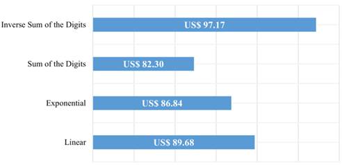
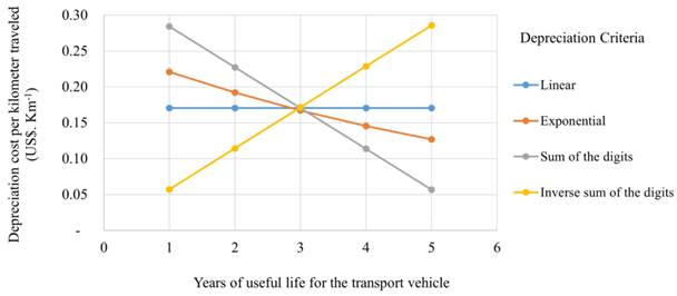
The criteria that yielded the lowest depreciation quotas at the end of the asset’s useful life (year 5) - and, consequently, a scenario of lower operating and per-kilometer costs - were Sum of the Digits, Exponential, and Linear, in that order (Figure 1 and Figure 2). Figure 2 shows the depreciation cost per kilometer for all four criteria, considering an estimated useful life of five years. As expected, during the first two years the criteria with the highest depreciation values were Sum of the Digits and Exponential. In the third year, depreciation values converged, with only minor differences among criteria. From the third year onward, the Inverse Sum of the Digits method produced the highest depreciation values.

Figure 1
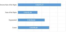
Influence of depreciation criteria on the operational cost of the forestry transport vehicle, evaluated in the fifth year of useful life.

Figure 2
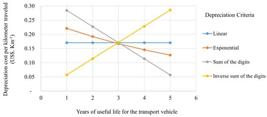
Behavior of depreciation cost per kilometer for the evaluated criteria throughout the estimated useful life of the forestry transport vehicle.

Depreciation curves for Sum of the Digits (Cole) and Exponential methods displayed similar behavior. In both cases, depreciation was more pronounced in the early years and tended to stabilize in the final years of the useful life of the asset, confirming the pattern reported by FREITAS et al. (2007). The Inverse Sum of the Digits method, however, showed the opposite trend: lower depreciation in the early years and progressive increases over time (Figure 2).

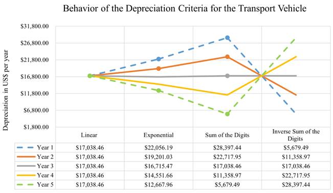
The Exponential and Sum of the Digits methods, which presented the lowest depreciation charges at the end of the asset’s useful life (Figure 3), proved to be more consistent for predicting depreciation behavior. REZENDE & VALVERDE (1997) also identified the Sum of the Digits method as an efficient approach for estimating asset depreciation. Although, the depreciation patterns varied across the criteria throughout the vehicle’s useful life, the overall balance among methods was similar. It is important to note; however, that different depreciation profiles affect the current asset value, which may influence annual tax and insurance costs, since these components are calculated by applying a rate to the current value of the asset. Selection of depreciation criteria in this study was arbitrary, and companies are advised to conduct preliminary analyses to identify the most appropriate criteria for their specific fleet conditions. Among the selected methods, those producing the most suitable estimates can be validated through comparison with accounting data or actual depreciation records.

Figure 3
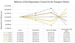
Behavior of depreciation costs for the forestry transport vehicle under the evaluated criteria, considering a five-year useful life.

Risk analysis

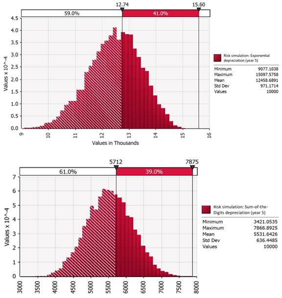
Using the Monte Carlo technique, simulations of possible depreciation scenarios were generated for the Sum of the Digits and Exponential methods, along with their associated cumulative probabilities (Figure 4). Annual depreciation values in year 5 that exceeded the calculated deterministic values were characterized as risks. Based on the simulations, there was a 39.00% and 41.00% probability of obtaining annual depreciation values above the calculated values for the Sum of the Digits and Exponential methods, respectively. Such high risk levels may pose challenges for forestry road transport operations, particularly when they affect cost components with strong influence on operational cost, as is the case with depreciation (FREITAS et al., 2004). As noted by SECURATO (2007), when uncertainty or risk is present, its probability must be quantified to support more assertive decision-making. Given the numerous variables involved and the excessive costs inherent to forestry road transportation, risk analysis is highly relevant for the activity (VIRGENS et al., 2021).

Figure 4
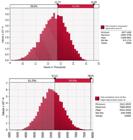
Probability distributions for Exponential and Sum of the Digits depreciation in year five, illustrating the risks of obtaining values higher than those determined.

Analysis of regression coefficients

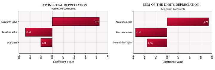
Analysis of the regression coefficients showed that depreciation values for the Sum of the Digits and Exponential methods in year 5 were significantly and positively influenced by the acquisition value of the forestry transport vehicle. In contrast, residual value and estimated useful life exhibited significant and inverse relationships with depreciation cost (Figure 5). According to the model, a 10% increase in the vehicle’s acquisition value would result in a 7.4% and 8.5% increase in depreciation for the Sum of the Digits and Exponential methods, respectively. Regarding estimated useful life, a 10% increase in this variable would lead to a 2.1% decrease in depreciation under the Exponential method (Figure 5). The asset’s service life is recognized as an influential factor in determining depreciation values (BALAKRISHNAN et al., 2004).

Figure 5
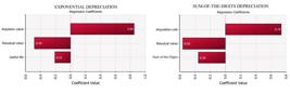
Regression coefficients for the input variables used in the risk analysis, considering the Exponential and Sum of the Digits depreciation criteria.

CONCLUSION

The depreciation criteria evaluated exhibited distinct behaviors throughout the forestry transport vehicle’s estimated useful life. However, their overall long-term balance was essentially equivalent. Among the methods, the Exponential and Sum of the Digits criteria proved to be the most consistent in predicting the actual depreciation of the evaluated vehicle. The magnitude of the risk identified in this study expressed as the probability of obtaining depreciation charges above the calculated value revealed a point of vulnerability for the forestry sector, particularly because depreciation represents a substantial portion of operational costs in road transportation systems. The risk modeling approach applied to asset depreciation demonstrated strong potential for supporting economic and sustainable planning in the forestry sector.

ACKNOWLEDGMENTS

To the Conselho Nacional de Desenvolvimento Científico e Tecnológico CNPq) for granting a Postdoctoral fellowship (Process No. 101806/2024-8).

To the Fundação de Amparo à Pesquisa do Estado da Bahia (FAPESB) and the Coordenação de Aperfeiçoamento de Pessoal de Nível Superior (CAPES) for awarding Master’s scholarships in Forest Sciences.

To Kemele Cristina Coelho for providing the data from her dissertation, which supported the development of this study.

REFERENCES

• BALAKRISHNAN, R. et al. A Resource granularity framework for estimating opportunity costs. Accounting Horizons, v.18, n.3, p.197-206, 2004. Available from: <Available from: https://publications.aaahq.org/accounting-horizons/article-abstract/18/3/197/1754/A-Resource-Granularity-Framework-for-Estimating?redirectedFrom=fulltext >. Accessed: Aug. 05, 2025. doi: 10.2308/acch.2004.18.3.197.
  » https://doi.org/10.2308/acch.2004.18.3.197.» https://publications.aaahq.org/accounting-horizons/article-abstract/18/3/197/1754/A-Resource-Granularity-Framework-for-Estimating?redirectedFrom=fulltext
• BERGER, R. et al. Minimização de custos de transporte florestal com a utilização da programação linear. Revista Floresta, v.33, p.54-55, 2003. Available from: <Available from: https://revistas.ufpr.br/floresta/article/view/2277 >. Accessed: Mar. 2, 2026. doi: 10.5380/rf.v33i1.2277.
  » https://doi.org/10.5380/rf.v33i1.2277.» https://revistas.ufpr.br/floresta/article/view/2277
• CHICHORRO, J. F. et al. Custos e índices econômicos de povoamentos de eucalipto do Programa Produtor Florestal no Espírito Santo. Pesquisa Florestal Brasileira, v.37, n.92, p.447-456, 2017. Available from: <Available from: https://pfb.sede.embrapa.br/pfb/article/view/1232 >. Accessed: Jun. 22, 2024. doi: 10.4336/2017.pfb.37.92.1232.
  » https://doi.org/10.4336/2017.pfb.37.92.1232.» https://pfb.sede.embrapa.br/pfb/article/view/1232
• CORDEIRO, S. A. et al. Contribution of the public promotion of a forest of Minas Gerais in returns and risk reduction for rural producers. Revista Árvore, v.34, n.32, p.367-376, 2010. Available from: <Available from: https://doi.org/10.1590/S0100-67622010000200020 >. Accessed: Jun. 22, 2024. doi: 10.1590/S0100-67622010000200020.
  » https://doi.org/10.1590/S0100-67622010000200020.» https://doi.org/10.1590/S0100-67622010000200020
• DINIZ, C. C. C. et al. Análise técnica e de custos do transporte de biomassa florestal com carreta piso móvel. Agropecuária Científica no Semiárido (ACSA), v.16, n.1, p.34-38, 2020. Available from: <Available from: https://acsa.revistas.ufcg.edu.br/acsa/index.php/ACSA/article/view/1118 >. Accessed: Mar. 15, 2023, doi: 10.30969/acsa.v16i1.1118
  » https://doi.org/10.30969/acsa.v16i1.1118» https://acsa.revistas.ufcg.edu.br/acsa/index.php/ACSA/article/view/1118
• FREITAS, L. C. et al. Comparative study of three methods for calculating operational cost of Bitrem truck. Revista Árvore, v.28, n.6, p.855-863, 2004. Available from: <Available from: https://www.scielo.br/j/rarv/a/LQgcYRQFrSj3FM3YKR43b6n/?lang=pt >. Accessed: Feb. 20, 2023. doi: 10.1590/S0100-67622004000600010.
  » https://doi.org/10.1590/S0100-67622004000600010.» https://www.scielo.br/j/rarv/a/LQgcYRQFrSj3FM3YKR43b6n/?lang=pt
• FREITAS, L. C. et al. Influence of methods for calculating depreciation on the income tax and cash flow of a forest transportion activity. Revista Árvore, v.31, n.2, p.257-264, 2007. Available from: <Available from: https://www.scielo.br/j/rarv/a/JxkRxwvXywpGQgryz3g8PhB/?lang=pt >. Accessed: Feb. 20, 2023. doi: 10.1590/S0100-67622007000200008.
  » https://doi.org/10.1590/S0100-67622007000200008.» https://www.scielo.br/j/rarv/a/JxkRxwvXywpGQgryz3g8PhB/?lang=pt
• MACHADO, A. K. T.; PAPARAZZO, L. G. Depreciação: estudo sobre conceito, aspectos e métodos de cálculo. Múltiplo Saber. 2025Available from: <Available from: https://www.inesul.edu.br/revista/arquivos/arq-idvol_29_1396385728.pdf >. Accessed: Aug. 23, 2025.
  » https://www.inesul.edu.br/revista/arquivos/arq-idvol_29_1396385728.pdf
• MACHADO, C. C. et al. Elementos básicos do transporte florestal rodoviário. Viçosa, MG. Editora UFV. 2005.1 ed., 167p.
• MARQUES, G. M. et al. Application of dynamic programming in equipment substitution. Revista Árvore, v.29, n.5, p.749-756, 2005. Available from: <Available from: https://www.scielo.br/j/rarv/a/gZYfS5VpY7yXLVXtS3jqg3r/?lang=pt >. Accessed: Aug. 23, 2025. doi: 10.1590/S0100-67622005000500010.
  » https://doi.org/10.1590/S0100-67622005000500010.» https://www.scielo.br/j/rarv/a/gZYfS5VpY7yXLVXtS3jqg3r/?lang=pt
• MOREIRA, J. M. M. et al. Impact of Transportation cost on forest risk and profitability in the region of Itapeva, São Paulo. Revista Paranaense de Desenvolvimento - RPD, v.38, n.132, p.77-89, 2017. Available from: <Available from: https://www.alice.cnptia.embrapa.br/alice/bitstream/doc/1073110/1/2017JoseMRPDImpacto.pdf >. Accessed: Mar. 02, 2026.
  » https://www.alice.cnptia.embrapa.br/alice/bitstream/doc/1073110/1/2017JoseMRPDImpacto.pdf
• PINTO, A. K. C.; OLIVEIRA, P. A. Análise da depreciação de veículos nacionais por faixa de preço. Tekhne e Logos, v.10, n.1, p.2-13, 2019. Available from: <Available from: http://revista.fatecbt.edu.br/index.php/tl/article/view/620 >. Accessed: Mar. 15, 2023.
  » http://revista.fatecbt.edu.br/index.php/tl/article/view/620
• REZENDE, J. L. P.; VALVERDE, S. R. Princípios de depreciação de máquinas e equipamentos. Revista Árvore, v.21, n.1, p.99-111, 1997.
• SAMPAIO, I. S. et al. Influence of the depreciation method on the wood transport cost. Ciência Florestal, v.31, n.1, p.145-156, 2021. Available from: <Available from: https://periodicos.ufsm.br/cienciaflorestal/article/view/32812 >. Accessed: Mar, 11, 2023. doi: 10.5902/1980509832812.
  » https://doi.org/10.5902/1980509832812.» https://periodicos.ufsm.br/cienciaflorestal/article/view/32812
• SECURATO, J. R. Decisões financeiras em condições de risco. São Paulo: São Paulo, 2007. 264 p.
• SILVA, E. N. et al. Evaluation of costs of two harvester models in the cut of Eucalyptus Ciência Florestal, v.24, n.3, p.741-748, 2014. Available from: <Available from: https://www.researchgate.net/publication/290526486_Evaluation_of_costs_of_two_Harvester_models_in_the_cut_of_Eucalyptus >. Accessed: Aug. 03, 2025. doi: 10.1590/1980-509820142403021.
  » https://doi.org/10.1590/1980-509820142403021.» https://www.researchgate.net/publication/290526486_Evaluation_of_costs_of_two_Harvester_models_in_the_cut_of_Eucalyptus
• SILVA, M. H. Economia da exploração florestal: estudo de caso do custo de transporte florestal no município de Rio Branco, 2013. I Prêmio Serviço Florestal Brasileiro em Estudos de Economia e Mercado Florestal. p.95.
• SIMÕES, M. Contabilidade mal explicada: o método de Cole. Imaginário Puro. 2018. Matemática aplicada. Online. Available from: <Available from: https://imaginariopuro.wordpress.com/2018/01/19/contabilidade-mal-explicada-o-metodo-de-cole/ >. Accessed: Mar. 11, 2023.
  » https://imaginariopuro.wordpress.com/2018/01/19/contabilidade-mal-explicada-o-metodo-de-cole/
• SOARES, A. P.; GABRIEL, B. R. J. Análise de Custos. Salvador, BA. UFBA, Faculdade de Ciências Contábeis; Superintendência de Educação a Distância, 2019.
• SOUZA, J. L. M.; FRIZZONE, J. A. Modelo aplicado ao planejamento da cafeicultura irrigada. III Análise de risco econômico da cafeicultura em dois sistemas de irrigação. Acta Scientiarum Agronomy, v.25, n.2, p.399-408, 2003. Available from: <Available from: https://periodicos.uem.br/ojs/index.php/ActaSciAgron/article/view/2455 >. Accessed: Aug. 05, 2025. doi: 10.4025/actasciagron.v25i1.2455.
  » https://doi.org/10.4025/actasciagron.v25i1.2455.» https://periodicos.uem.br/ojs/index.php/ActaSciAgron/article/view/2455
• VIRGENS, A. P. et al. M. L. Economic assessment and risk management for different distances of timber transport by road. Ciência Florestal, v.31, n.2, p.880-897, 2021. Available from: <Available from: https://periodicos.ufsm.br/cienciaflorestal/article/view/35470 >. Accessed: Aug. 20, 2024. doi: 10.5902/1980509835470.
  » https://doi.org/10.5902/1980509835470.» https://periodicos.ufsm.br/cienciaflorestal/article/view/35470
• WILLIAMSON, G.; NIEUWENHUIS, M. Integrated timber allocation and transportation planning in Ireland. Journal of Forest Engineering, v.5, n.1, p.7-15, 1993. Available from: <Available from: https://www.tandfonline.com/doi/abs/10.1080/08435243.1993.10702649 >. Accessed: Aug. 03, 2025. doi: 10.1080/08435243.1993.10702649.
  » https://doi.org/10.1080/08435243.1993.10702649.» https://www.tandfonline.com/doi/abs/10.1080/08435243.1993.10702649

• CR-2025-0156.R1
• DATA AVAILABILITY STATEMENT
  The datasets generated and/or analysed during the current study are available from the corresponding author on reasonable request.
• DECLARATION OF USE OF ARTIFICIAL INTELLIGENCE
  We declare that no artificial intelligence resources were used in the writing or development of this manuscript.

Edited by

• ASSOCIATE EDITOR:
  Alessandro Dal’Col Lúcio (0000-0003-0761-4200)

• SCIENTIFIC EDITOR:
  Janaína Balk Brandão (0000-0002-3044-3473)

Data availability

The datasets generated and/or analysed during the current study are available from the corresponding author on reasonable request.

Publication Dates

• Publication in this collection
  27 July 2026
• Date of issue
  2026

History

• Received
  20 Mar 2025
• Accepted
  08 Dec 2025
• Reviewed
  04 May 2026